Valid Rules of Inference, Part 1 (Inferences From Conditional Statements)

1. Rules of Inference

We saw in the previous tutorial that a logic proof is essentially an argument where we “show our work,” and that this entails referencing rules that justify each derivation, or step in our reasoning. As you know, these are called rules of inference. We will learn eight of these rules in this class, which will be sufficient to construct many proofs. There is some disagreement among logicians about how many basic rules of inference there are, and an exhaustive list of rules could number around forty and is beyond the scope of the class. These eight will suffice for our purposes and are the classic rules for sentential logic.

In this tutorial, you will learn three rules of inference that pertain to conditional sentences; these three will be found on anyone’s list of basic rules of inference.

hint

While in everyday use, we may call an educated guess an “inference,” in logic, the word guarantees logical certainty. If you can logically infer one statement from another, then it necessarily follows. It is important to keep these technical meanings distinct from more casual usage and avoid the fallacy of equivocation.

---

2. Conditional Elimination (Modus Ponens)

The rules of inference need to be so clear and straightforward that they are acceptable in themselves, or our proofs wouldn’t prove anything. In fact, some may seem so obvious that you’d wonder why they need a name at all. For example, take this argument:

1. p → q
2. p
3. ∴q

The argument assumes two premises: 1) If p, then q; and 2) p is true. It concludes that q is true. This is a classic rule of inference called Conditional Elimination. Originally in Latin it is called Modus Ponens.

What this form says, in words, is that if we have a conditional sentence (p → q), and we have established that the antecedent of that conditional sentence (p) is true, then we can conclude a stand-alone sentence declaring that the consequent (q) is true. We “eliminate” the conditional from the sentence, hence the name of the rule.

For example, take these statements:

1. If it is raining, then the ground is wet.
2. It is raining.
3. Therefore, the ground is wet.

The conclusion logically follows, and we can use “the ground is wet” to support any further arguments. Say the argument continued:

4. If the ground is wet, I don’t have to water.
5. Therefore, I don’t have to water.

The conclusion here is itself derived using Conditional Elimination, but it is first necessary to derive “the ground is wet” to reach that conclusion. Notice that in the full argument 1–5, we actually have two instances of Conditional Elimination that allow us to conclude statement 5.

As with any rule of inference, we can show that Conditional Elimination is valid by constructing a truth table. As you can see below, in the only row where both premises are true, the conclusion is also true.

p	q	p → q	p	q
T	T	T	T	T
F	T	T	F	T
T	F	F	T	F
F	F	T	F	F

Recall that we have used propositional variables to represent this rule, because the rule holds for any logical sentence, atomic or complex. The propositional variables may themselves represent disjunction, conjunctions, or even conditional sentences. Consider this example:

1. (A ∧ B) → C
2. A ∧ B
3. ∴ C

In this argument, we can conclude C because of the rule of Conditional Elimination. Here is what Conditional Elimination would look like in a proof.

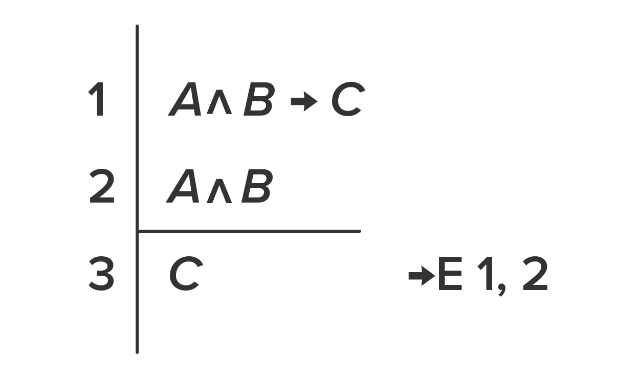
You can see that this is the same argument as above, but now in proof form, with a line demarcating the premises and the conclusion, and a notation on the right that explains what rule we are applying. Each notation will always have two parts.

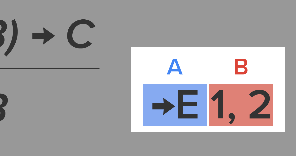
In line 3, the first part of the notation is the rule we are applying. In this example, →E means “Conditional Elimination.” The symbol, →, is shorthand for “conditional,” (because that is its logical meaning, as we know). The E stands for elimination, which in the terms of a proof means reduction of a complex sentence to a less complex sentence.

The second part of the notation is the number(s) of previous statements we are applying that rule to. Many rules of inference, like this one, apply to exactly two earlier steps in the proof.

key concept

→E

The notation used in a proof when the rule of Conditional Elimination has been applied to derive the new sentence.

term to know

Conditional Elimination (also known as Modus Ponens)

A rule of inference stating that if we have a conditional sentence (p → q) and we have established that the antecedent (p) is true, then we are licensed to infer that the consequent (q) is true.

---

3. Modus Tollens

The next form of inference is called Modus Tollens (MT), which is again a Latin phrase, this time meaning “denying the consequent.” As with Modus Ponens (Conditional Elimination), it’s easy to confuse this rule with the two logical fallacies we discussed earlier, but Modus Tollens is completely valid. It looks like this:

1. p → q
2. ¬q
3. ∴¬p

What this rule says, in words, is that if we have a conditional sentence (p → q) and we have established that the consequent is false (¬q), then we can add a sentence to the proof declaring that the antecedent is false (¬p).

Take this example:

1. If it is raining, then the ground is wet.
2. The ground is not wet.
3. It is not raining.

Perhaps in this instance, the argument continues:

4. If it is not raining, I can go for my run.
5. Therefore, I can go for my run.

As before, the main conclusion (step 5) cannot be derived without first deriving the statement, “It is not raining.” That’s why proofs are useful—they allow us to follow or illustrate a chain of derivations. In this class, we will only call this rule Modus Tollens, using the shorthand MT, plus the numbers of the statements/sentences to which it is applied.

Let’s think about why the reasoning for this rule makes sense. Consider the first half of our argument from above (1–3). If we know that the conditional “if it is raining, then the ground is wet” is true, then we know two things about the relationship between rain and ground wetness. First, rain always causes ground wetness. Anytime it is raining, the ground necessarily will be wet. Second, without ground wetness there can be no rain (ground wetness is necessary for rain). This is the best way to understand Modus Tollens. The conditional plus the fact that there is no ground wetness means there can’t possibly be rain.

key concept

MT

The notation used in a proof to show the rule of Modus Tollens has been applied to derive the new sentence.

As you can see from the truth table, Modus Tollens will always be true, regardless of the meanings of p and q, because in the one case where the premises are both true, the conclusion is also true. And as with Conditional Elimination, the p and q are propositional variables that can stand for any complex sentence.

p	q	p → q	p	q
T	T	T	F	F
F	T	T	F	T
T	F	F	T	F
F	F	T	T	T

term to know

Modus Tollens

A rule of inference stating that if we have a conditional sentence (p → q) and have determined the consequent is false (¬q), then we are licensed to infer that the antecedent is false (¬p).

---

4. A Review of Conditional Statements and Inference

You can see that Modus Tollens is closely connected to Conditional Elimination, and both are closely related to two logical fallacies we learned earlier. Indeed, all four have to do with conditional sentences and what we can infer when we know the truth value of either the antecedent or the consequent. However, we can only validly infer anything if we know (a) that the antecedent is true, or (b) that the consequent is false.

	…Antecedent	…Consequent
Affirming the…	Valid (Conditional Elimination) p → q p ∴q	Fallacy (Affirming the Consequent) p → q q ∴p
Denying the…	Fallacy (Denying the Antecedent) p → q ¬p ∴¬q	Valid (Modus Tollens) p → q ¬q ∴¬p

---

5. Using Conditional Elimination and Modus Tollens in a Proof

We will now build a proof using the two rules we’ve learned, Conditional Elimination (→E) and Modus Tollens (MT). First, here is the argument.

1. (R ∨ S) → (T → K)
2. ¬K
3. R ∨ S
4. ∴ ¬T

This is a valid argument, but the reason it is valid is probably not so easy to see at a glance, and even harder to explain to someone else. This is where proofs come in handy!

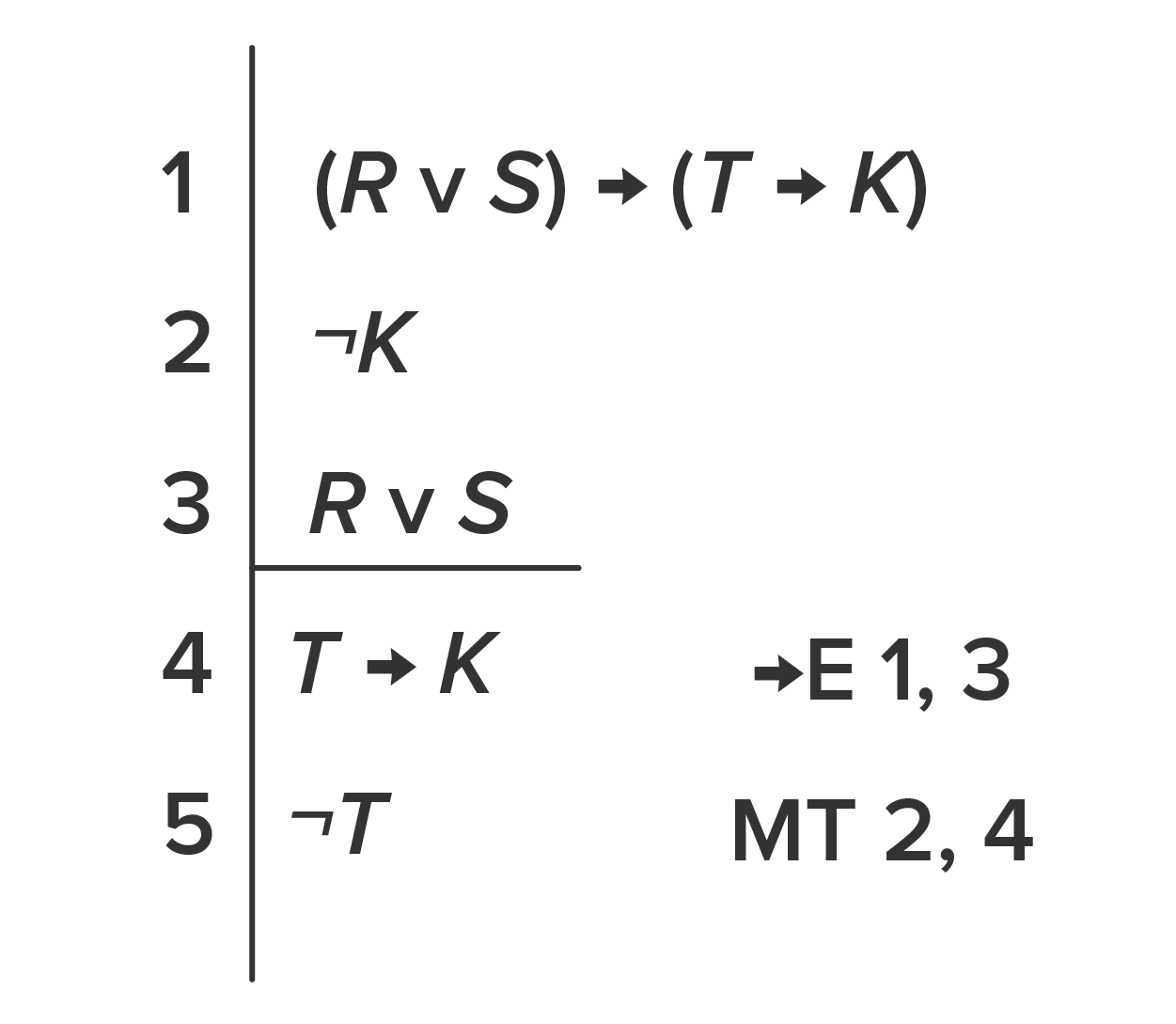
You now know how to interpret the notations on the right. Sentence 4 is true because the rule of Conditional Elimination is applied to sentences 1 and 3. Notice that sentence 3, (R ∨ S), is the antecedent of the conditional in sentence 1. Thus, we can use Conditional Elimination to conclude the consequent of the conditional. Sentence 4 and sentence 2 are then used to derive sentence 5, applying the rule Modus Tollens to lines 2 and 4. Line 2 is a negation of the consequent of the conditional in sentence 4, and so we can conclude the negation of the antecedent, line 5. ¬T is the conclusion we’re trying to reach, so the proof is completed.

---

6. Conditional Introduction

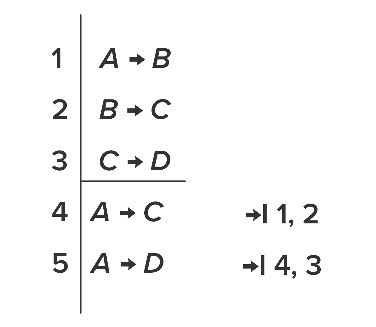
We will learn one more rule of inference related to conditional sentences. First, let’s see what it looks like in logical form.

1. p → q
2. q → r
3. ∴ p → r

All three sentences are conditionals, and the conclusion is derived from the first two by linking them together; we can say that p leads to r because p leads to q and q leads to r. This rule of inference is called Conditional Introduction because we are introducing a new conditional sentence to the proof. The essence of the rule is that if two conditional sentences are linked, meaning the consequent of the first is the antecedent of the second, we can add a new conditional sentence to the proof eliminating the redundant sentence that the two conditionals have in common.

A brief history lesson. You may hear the term hypothetical syllogism in reference to this last rule. The term syllogism comes from categorical logic (the logical system created by Aristotle around 350 BCE) and refers to an argument where the conclusion is derived via deductive reasoning from exactly two premises. (If it is derived from one premise, you may recall, it is a tautology.) The classic example of this is the argument:

1. All men are mortal.
2. Socrates is a man.
3. Therefore, Socrates is mortal.

As we mentioned earlier, the term hypothetical refers to conditional statements. As a technical term, “hypothetical syllogism” is another name for the Conditional Introduction rule, though we won’t use that term.

big idea

Many rules of inference are also syllogisms, including Modus Tollens, Conditional Elimination, and Conditional Introduction.

Let’s use an example to understand conceptually why this rule works the way it does. Consider the following argument:

1. If it is raining, then the ground is wet.
2. If the ground is wet, then the roads are slippery.
3. ∴ If it is raining, then the roads are slippery.

Premise 1 states that ground wetness always accompanies rain and premise 2 says that road slipperiness always accompanies ground wetness. So, any time we have ground wetness, we automatically have road slipperiness, and anytime we have rain, we automatically have ground wetness. Hence, not only is rain accompanied by ground wetness, but it’s also accompanied by road slipperiness. And that is how we get our conclusion: if it’s raining, then the roads are slippery.

Let’s see the validity of Conditional Introduction in a truth table.

p	q	r	p → q	q → r	p → r
T	T	T	T	T	T
F	T	T	T	T	T
T	F	T	F	T	T
F	F	T	T	T	T
T	T	F	T	F	F
F	T	F	T	F	T

If you check each of the rows in which the premises (columns 4 and 5) are true, the conclusion (column 6) is also true. Thus, Conditional Introduction is valid.

Theoretically, we can have as many premises as we want and the conclusion would still be valid, as long as each consequent becomes an antecedent in the next conditional sentence before the conclusion. For this reason, the rule is sometimes referred to as “the chain argument.”

1. p → q
2. q → r
3. r → s
4. s → t
5. ∴ p → t

However, when writing the proof for this argument, we may not simply derive the conclusion p → t and justify it by citing Conditional Introduction and premises 1–4. We must first show that each intermediate derivation is legitimate: that p → r, then that p → s, then that p → t. If the chain continued, so would our proof! Conditional Introduction is notated as →I, followed by the two sentences it applies to. Remember, Conditional Introduction is a syllogism, so it cannot apply to more than two sentences in a proof. Hence, we work through every intermediate step.

key concept

→I

The notation used in a proof to show the rule of Conditional Introduction has been applied to derive the new sentence.

terms to know

Conditional Introduction (also called Hypothetical Syllogism)

A rule of inference stating that if two conditional sentences are linked, meaning the consequent of one is the antecedent of the other (p → q, q → r), we are licensed to infer the truth of a new conditional sentence with the antecedent from the first sentence and the consequent of the second (p → r).

Syllogism

A deductive argument where the conclusion is derived from two premises.