Table of Contents |
The graph you see here is that of a standard, normally distributed variable, otherwise known as a z-distribution. Because they allow you to know the position of a value in a normal distribution, z-scores are important. When you know a z-score associated with the value of a variable, you are able to determine the likelihood that an event will take place. Simply having a solid understanding of z-scores and how they are associated with probability allows you to easily determine the likelihood of an event occurring.
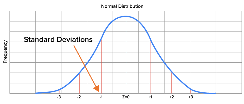
Approximately 68% of values in a normally distributed variable fall between a z-score of -1 and 1. Ninety-five percent of values fall between a value of -2 and 2; 99.7% of values fall between a z-score of -3 and 3. If you were to think of likely values in a normal distribution, they would fall in the 95% between a z-score of -2 and 2.
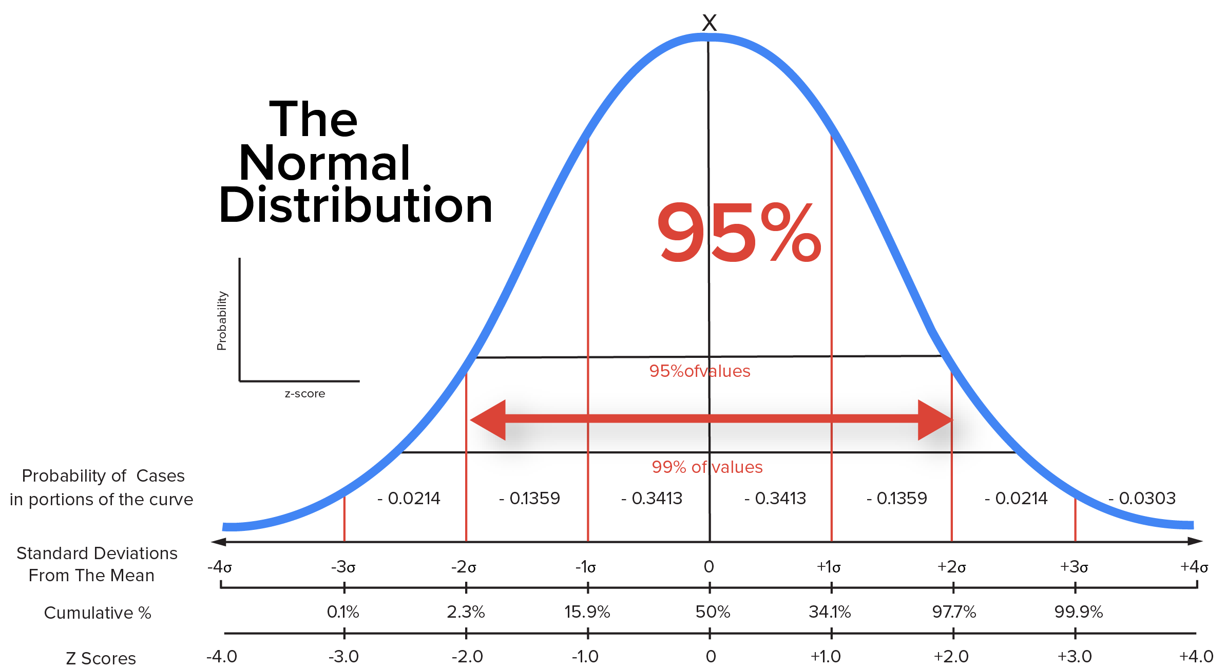
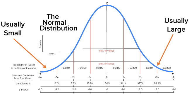
If a value has a large positive z-score, you would consider it to be unusually large, and not very likely to occur. Along the same line of thought, if a value has a large negative z-score, you would consider it to be unusually small, and not very likely to occur either.
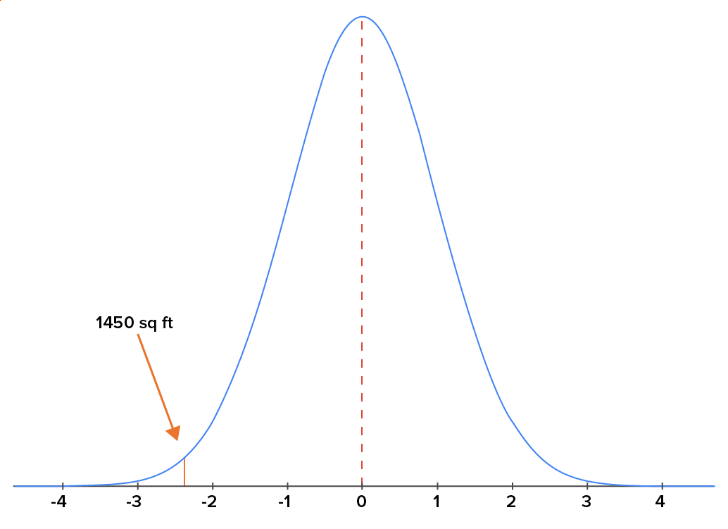
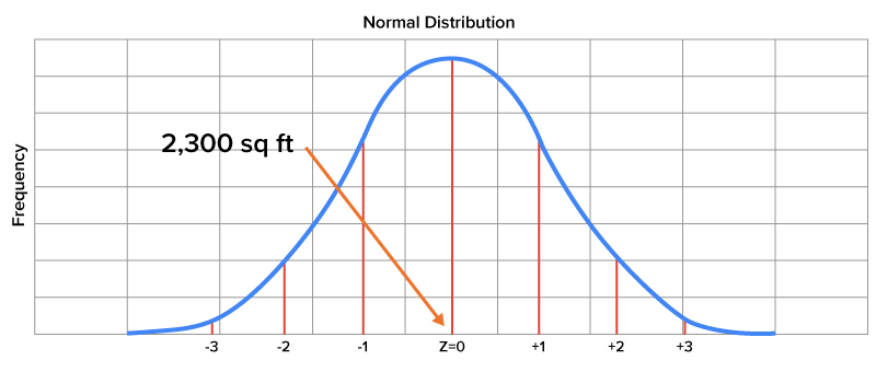
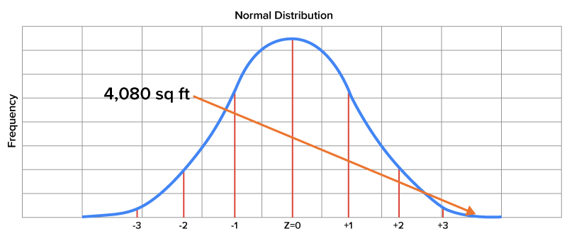
Suppose you were to take a look at the mean area of all homes in the United States in terms of square feet. Say that the mean area of a home in the United States is 2,400 square feet, with a standard deviation of 400 square feet. The table below shows multiple z-scores.
| Value | Z-Score | Graph |
|---|---|---|
| A home with area of 1,450 square feet |
z-score = 
|
|
| A home with area of 2,300 square feet |
z-score = 
|
|
| A home with area of 4,080 square feet |
z-score = 
|
|
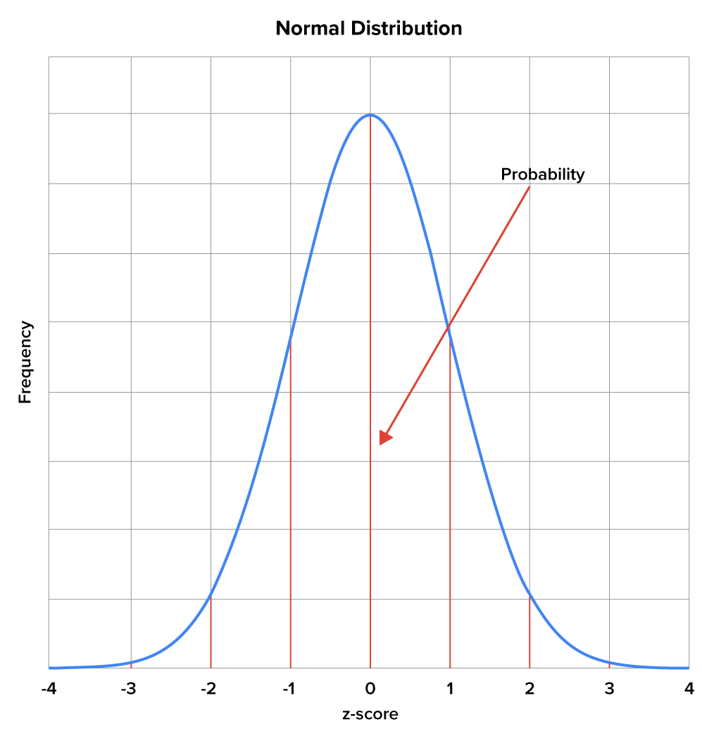
When viewing a normal distribution graph, the area under the curve is associated with the probabilities of a value occurring. Knowing the area corresponding to a z-score tells us about the probability of an event taking place.
Notice the organization of the z-tables below. The negative z-table starts out at the left of the distribution (-3) and shows increasing values of z up to the point of z being equal to 0. The positive z-table begins at the center of the z-distribution, where z is equal to 0 and represents the mean of the distribution.
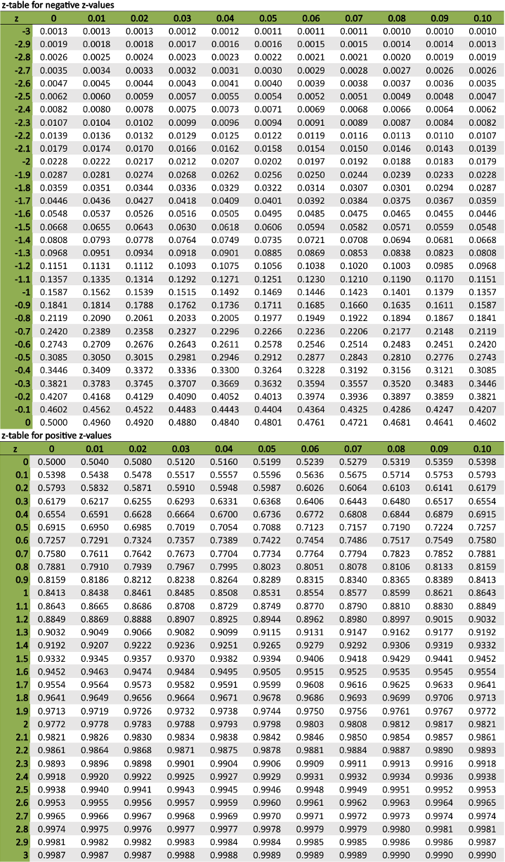
The values for both z-tables correspond with the same information that is illustrated in a z-distribution graph but actually say more about the specific likelihood of an event occurring.
If you are provided with a negative z-score, you use the negative z-table to find the area under the curve to the left of the given z-score. This area under the curve is equal to the proportion of all z-scores in this range. When you have a positive z-score, the positive z-table lets you find the area under the curve to the left of that given z-score. This area under the curve is equal to the proportion of all z-scores in this range.
Take a look at ACT scores to illustrate this. The American College Test, or ACT, is taken by high school students all across the United States as a means of determining their aptitude for attending college. Let’s suppose in this instance that the mean score for the population is 21, and the standard deviation in this case is 5. How will you determine the probability that a score would fall within a particular range?
Consider the probability that the score would be higher than 30. How do you determine what that value is? The first thing you do is use the z-score formula to figure out what the z-score is. In this case, it is the difference between 30 and 21, which is 9, divided by the standard deviation of 5, which gives you a z-score of 1.8. If you look at the z-table below, that gives you a probability value of 0.9641.
Probability of an ACT score > 30
Mean = 21
Standard Deviation = 5

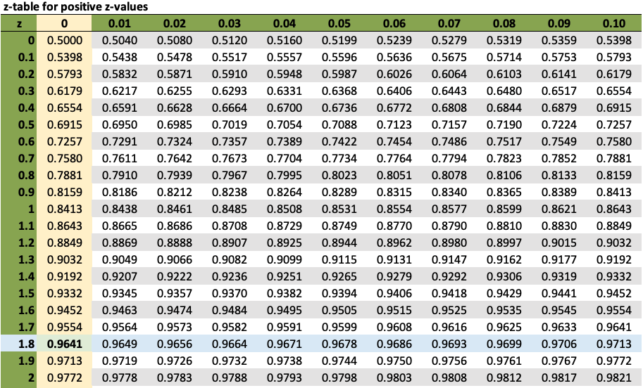
Now, what does that tell you? It tells you that the area to the left of that point is 0.9641, or roughly 96% of the area under the curve falls to the left of z equal to 1.8. To determine the probability that the score is greater than 30, you’re interested in the difference between 0.9641 and 1, which gives you a probability of 0.0359.

What if you’re interested in the probability that a score falls between 23 and 27? In this instance, you need to calculate two different z-scores, one for 23 and one for 27. Locate both of these z-scores on the z-table. Then subtract the difference between the greater value and the lower value. That is the probability that a randomly drawn score would fall between the range of 23 and 27.
Probability of a score between 23 and 27

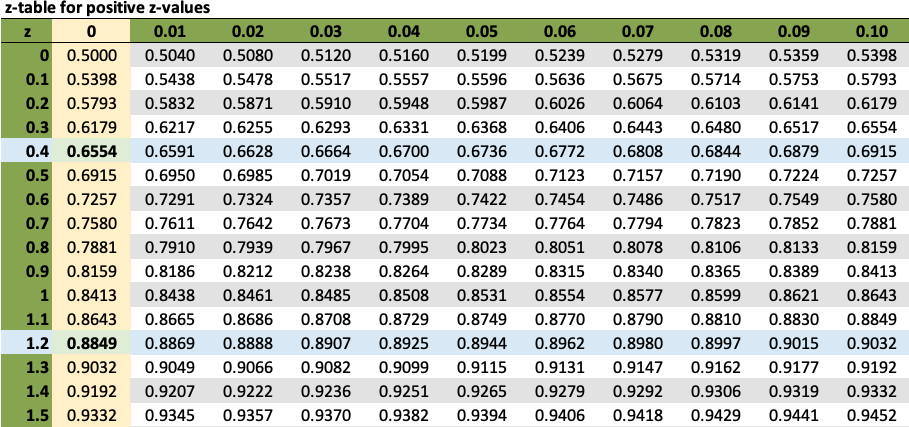
What if you’re looking at some areas to the left of the mean? Suppose you’re interested in the probability that a score falls between 15 and 20. You will run the same type of calculations. The z-score for a 20 would be equal to a negative 0.2. The z-score for 15 would be equal to negative 1.2. Once again, you figure out the probabilities associated with each value by finding the difference. This works out to be a probability of 0.3056.
Probability of a score between 15 and 20

Lastly, look at the probability that a score will be less than 20. Here you simply need to find the z-score for 20, which is equal to -0.20. The probability for this value is 0.4207, which tells you that’s the probability that a score would be below 20, based upon a normal distribution.
Probability of a score less than 20

What if you’re interested in determining the value of a variable based upon a predetermined probability? Hypothetically speaking, let’s look at the miles driven per year by the American driver. Say that in the population that you’re looking at, the mean miles driven per year is 16,550, with a population standard deviation of 2,100.
Suppose you were interested in finding the number of miles driven per year in which there were only 1.5% of all observations below that value. How do you determine that figure? Well, you establish your probability of 1.5%. Then, divide that by 100 to arrive at a probability equal to 0.015, which is the value you will look up in your z-table.
You scan through the numbers until you find the value that’s equal to 0.015, which is going to be in the negative side of the z-table. Look at the columns and the rows, and you will find the value of 0.015 happens to have a z-value of -2.17. Now, plug that into the z-score formula and solve for the value:

The result is 11,993 miles per year. Only 1.5% of drivers drive fewer than that number of miles per year.
Suppose that you have a probability of 69.5%. Once again, divide this value by 100 to arrive at a probability of 0.695, and scan the z-table to find that 0.695 value. It turns out that the z-value is equal to 0.51.
To solve for your value, you look at whatever the value is minus 16,550. We take the difference and divide it by 2,100 to get 0.51. So, if you do a little cross multiplication, you arrive at a value of 17,621 miles per year, in which case 69.5% of drivers would drive less than that.

Source: THIS TUTORIAL WAS AUTHORED BY DAN LAUB FOR SOPHIA LEARNING. PLEASE SEE OUR TERMS OF USE.