Two-Sample Hypothesis Testing for Means: Left-Tailed Test

1. Introduction to Two-Sample Hypothesis Tests for Means: Left-Tailed Tests

Two-sample hypothesis testing for means in left-tailed tests is a statistical method used to determine if the mean of one group is significantly less than the mean of another group. In this type of test, the null hypothesis states that the means of the two groups are equal, while the alternative hypothesis suggests that the mean of the first group is less than the mean of the second group. This approach is particularly useful when you want to test for reductions or decreases in a specific metric.

For example, suppose you want to analyze the impact of a cost-cutting measure. You could compare the average expenses from two different periods: one before the implementation of the measure and one after. The left-tailed test would help determine if the new measure has significantly reduced expenses. The null hypothesis would be that the average expenses before and after the measure are the same, and the alternative hypothesis being that the average expenses after the cost-cutting measure are lower.

1a. Applications of Two-Sample Hypothesis Tests for Means: Left-Tailed Tests

Let's walk through a practical example of performing a two-sample hypothesis test for means for a left-tailed test.

EXAMPLE

QuantumLeap IT is a mid-sized technology firm specializing in software development and IT consulting services. The company has been experiencing steady growth over the past few years, but recent economic challenges have prompted the management team to implement cost-cutting measures to maintain profitability and ensure long-term sustainability.

To evaluate the effectiveness of these cost-cutting measures, the finance department at QuantumLeap IT has decided to analyze the monthly expenses before and after the implementation of the measures. The goal is to determine whether the new measures have significantly reduced the company’s expenses.

The finance team collected monthly expense data for a sample of 50 expenses from several departments within the company. The data includes expenses for six months before the cost-cutting measures were implemented and six months after.

As the data analyst for QuantumLeap IT, you will perform a two-sample left-tailed hypothesis test to compare the average expenses before and after the cost-cutting measures.

Step 1: State the Hypotheses

• H₀: (mean expenses before and after the cost-cutting measures are the same)
• H₁: (mean expenses after the cost-cutting measures are lower than the average expenses before)

Step 2: Gather the Data

Expense data was randomly sampled for 50 different expenses from several different departments across the company before and after the cost-cutting measures were put in place. The data is in the Excel file named expenses_before_after_cost_cutting.xlsx.

Step 3: Choose a Significance Level

Use a level of significance,

Step 4: Check for Equal Variances

You test the following in Excel:

• H₀: (variances in the expense data before and after the cost-cutting measure are equal)
• H₁: (variances in the expense data before and after the cost-cutting measure are not equal)

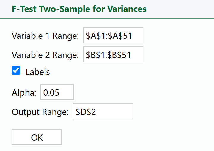
To perform the equality of variances test in Excel using the expenses_before_after_cost_cutting.xlsx file, perform the following:

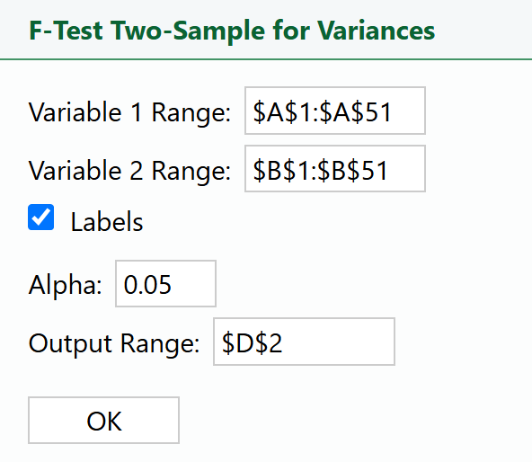
1. Select F-Test Two Sample for Variances in the XL Miner Analysis Toolpak. The dialog box opens.



2. Place your cursor in the Variable 1 Range: box and select the data in column A.

3. Place your cursor in the Variable 2 Range: box and select the data in column B.

4. Place your cursor in the Output Range: box, select cell D2 in the Excel worksheet, and select OK.



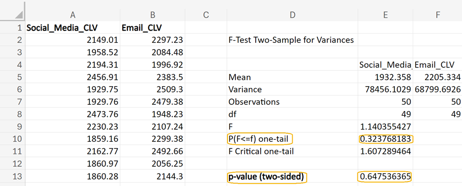
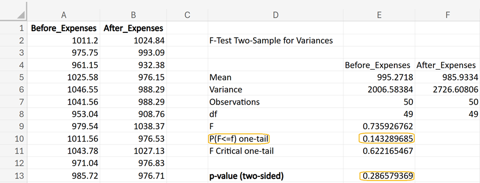
From Excel, you obtain the following output. In cell E13, you can enter =2*E10 to obtain the 2-sided p-value for this test. This p-value (0.2866) is greater than the level of significance of 0.05, so you fail to reject the null hypothesis.

This result means there is not enough evidence to conclude that the variances of the expenses before and after the cost-cutting implementation are different. In other words, the variances are considered equal for the purposes of selecting the appropriate two-sample t-test.



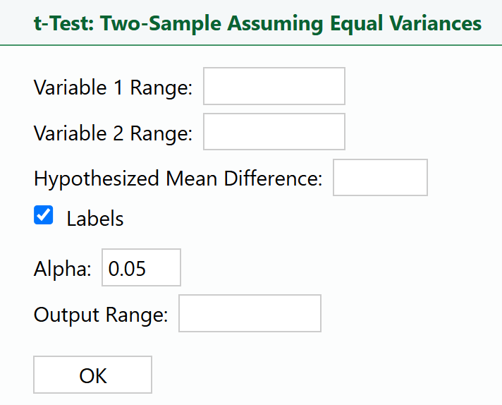
For the two-sample hypothesis test, you will select the t-Test: Two-Sample Assuming Equal Variances option in XL Miner.

Step 5: Perform a Statistical Test

You will now use the XL Miner Analysis Toolpak to find the p-value for this two-sample hypothesis test (left-tailed) using the data in the expenses_before_after_cost_cutting.xlsx Excel file.

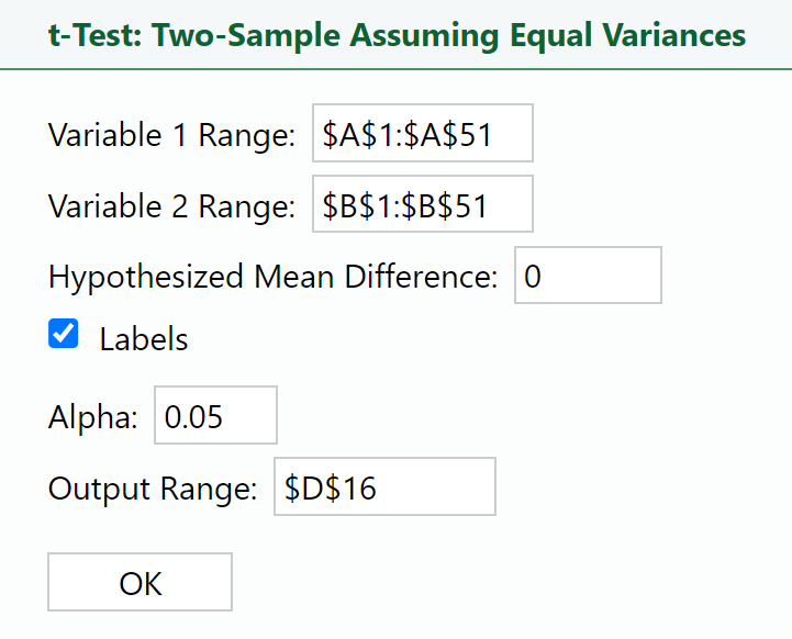
1. Select t-Test: Two-Sample Assuming Equal Variance in the XL Miner Analysis Toolpak. The dialog box opens.



2. Place your cursor in the Variable 1 Range: box and select the data in column B.

3. Place your cursor in the Variable 2 Range: box and select the data in column A.

4. Enter 0 in the Hypothesized Mean Difference: box.

5. Place your cursor in the Output Range: box, select cell D16 in the Excel worksheet, and select OK.



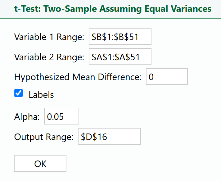
Notice in the dialog box above that the column in the Variable 1 Range specifies the data related to the sales after the marketing strategy was implemented, After_Expenses. Once again, the options you select for the Variable 1 and Variable 2 boxes in the t-test dialog box are crucial, because they directly determine the direction of your hypothesis test using the directional math operator in your alternative hypothesis.

The alternative hypothesis is:

H₁:

To set this alternative hypothesis up correctly in the t-test dialog box:

• Variable 1 Range: Select the range for After_Expenses (cells B2:B51).
• Variable 2 Range: Select the range for Before_Expenses (cells A2:A51).

By correctly setting the Variable 1 and Variable 2 ranges, you ensure that the test is aligned with your alternative hypothesis and that the results will accurately reflect whether the expenses after the cost-cutting measures are implemented are significantly less than the expenses before (Wright, n.d.).

Just like with the right-tailed test in the previous tutorial, the key is to make sure that whatever group is on the left-hand side of the mathematical operator in the alternative hypothesis is the group that is specified in the Variable 1 Range box.

The Hypothesized Mean Difference: option is usually set to 0. This option directly relates to the null hypothesis.

The null hypothesis is:

H₀:

It means we start by assuming there is no difference between the expenses before and after the cost-cutting measures. Another way to specify this is to say that the difference between the means of the two groups is zero. Subtract from both sides of the equation to obtain H₀: which we test against the alternative hypothesis that the expenses after the cost-cutting measures are less than the expenses before.

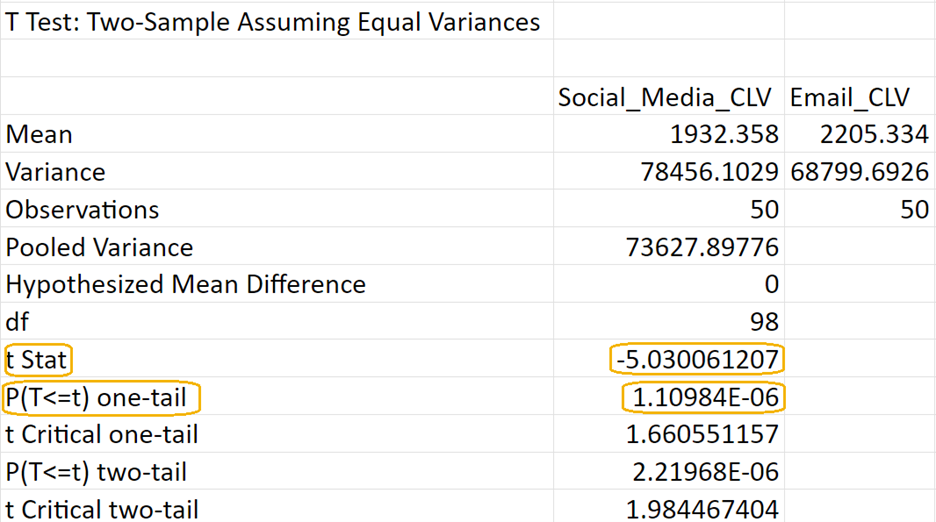
You will obtain the following output in your Excel worksheet. If the test statistic (row labeled t Stat) is negative, then the row labeled P(T<=T) one-tail is the left-tailed p-value. The p-value for this two-sample hypothesis test is 0.1698.



Below is a table to help you calculate the p-value for a left-tailed test based on the sign of the test statistic using the P(T <= t) one-tail output from the XL Miner Analysis ToolPak (Wright, n.d.):

Test Statistic	P(T<=t) one tail	Left-Tailed p-value Calculation
Positive	p	1-p
Negative	p	p

• Positive Test Statistic: If the test statistic is positive, you need to subtract the P(T <= t) one-tail value from 1 to get the left-tailed p-value.
• Negative Test Statistic: If the test statistic is negative, the P(T <= t) one-tail value is already the p-value for the left-tailed test.

Step 6: Make a Decision

Since the p-value (level of significance), you fail to reject the null hypothesis.

Step 7: Interpret the Results

Since the p-value (0.1698) is greater than the significance level (0.05), you fail to reject the null hypothesis. This means there is not enough statistical evidence to conclude that the cost-cutting measures have significantly reduced the company’s expenses.

In practical terms, for QuantumLeap IT, this result suggests that the cost-cutting measures implemented by the management team have not led to a statistically significant reduction in monthly expenses. The company may need to reassess these measures or consider additional strategies to achieve the desired cost savings.

The finance team may need to adjust future budgets and forecasts, considering that the expected savings from the cost-cutting measures were not realized. This could impact financial planning and resource allocation.

The results can inform broader strategic decisions. For instance, QuantumLeap IT might consider diversifying its services or entering new markets to boost revenue instead of focusing solely on cost reduction.

Now that you have explored the practical implications of the QuantumLeap IT expense cost-cutting example using a two-sample hypothesis testing approach, it is time for you to apply your knowledge by performing a two-sample hypothesis test using another real-world scenario!

In the next Try It exercise, you will work through the steps of a left-tailed test using a real-world business data analytics scenario.

try it

For the scenario provided, construct a two-sample t-test to address the business problem. Use a level of significance of 0.05. Ensure your solution contains:

1. A statement of the hypotheses.
2. A test for equality of variances.
3. An interpretation of what the result of the hypothesis test means in the context of the problem.

Innovatech Solutions, a rapidly growing tech startup specializing in cloud-based software solutions, is facing challenges in optimizing its marketing strategies. Innovatech Solutions is evaluating the effectiveness of two different marketing channels—social media and email—to determine which one results in higher Customer Lifetime Value (CLV). The company wants to test if the CLV from customers acquired through social media is less than those acquired through email marketing.

As a business data analyst at Innovatech Solutions, your task is to analyze the CLV data for customers acquired through social media and email channels and perform a two-sample t-test to determine if the average CLV from customers acquired through social media is less than the average CLV from customers acquired through email.

The Excel file CLV_marketing.xlsx contains a sample of 50 customers where each row represents the CLV value of an individual customer acquired through either the social media or email marketing channel. The data captures the Customer Lifetime Value (CLV) for each customer, rather than monthly data.

Solution:

The hypotheses are:

• H₀: (average CLV for customers acquired through social media is equal to CLV for customers acquired through email marketing)
• H₁: (average CLV for customers acquired through social media is less than the CLV for customers acquired through email marketing)

You need to perform the equality of variances test to determine which t-test you will select for the two-sample hypothesis test.

The hypotheses are:

• (variance in CLV for customers acquired through social media is equal to variance in CLV for customers acquired through email marketing)
• (variance in CLV for customers acquired through social media is not equal to variance in CLV for customers acquired through email marketing)

Use the F-Test Two-Sample for Variances option in the XL Miner Analysis Toolpak. Your options should look like:



From Excel, you obtain the following output. In cell E13, you can enter =2*E10 to obtain the 2-sided p-value for this test. This p-value is less than 0.6475, so you fail to reject the null hypothesis and conclude that the variances among the CLV values for both marketing channels are equal when selecting the appropriate two-sample t-test.



For the two-sample hypothesis test, you will select the t-Test: Two-Sample Assuming Equal Variances option in XL Miner.



You obtain the following output from Excel. If the test statistic (row labeled t Stat) is negative, then the row labeled P(T<=T) one-tail is the left-tailed p-value. The p-value for this two-sample hypothesis test is less than 0.0001.



Below is a table to help you calculate the p-value for a left-tailed test based on the sign of the test statistic using the P(T <= t) one-tail output from the XL Miner Analysis ToolPak:

Test Statistic	P(T<=t) one tail	Left-Tailed p-value Calculation
Positive	p	1-p
Negative	p	p

• Positive Test Statistic: If the test statistic is positive, you need to subtract the P(T <= t) one-tail value from 1 to get the left-tailed p-value.
• Negative Test Statistic: If the test statistic is negative, the P(T <= t) one-tail value is already the p-value for the left-tailed test.

Since the p-value (< 0.0001) is less than the significance level (0.05), you reject the null hypothesis. This means there is evidence to conclude that the mean CLV for customers acquired from social media channels is less than the mean CLV for customers acquired from email marketing campaigns.

watch

Check out this video on how to construct a two-sample t-test to evaluate the impact of two marketing channels on Customer Lifetime Value.

REFERENCES

Wright, D. (n.d.). Tail of the test: Interpreting Excel data analysis t-test output. Retrieved November 12, 2024, from www.drdawnwright.com/tail-of-the-test-interpreting-excel-data-analysis-t-test-output/.