The Normal Distribution

before you start

This lesson builds on key concepts from an Introduction to Statistics course. Specifically, we will cover the normal distributions, assuming familiarity with this foundational idea.

1. Introduction to the Normal Distribution

Suppose you are a business analyst at a retail store, and you have collected monthly sales data over the past year. You want to analyze this data to understand the sales pattern and find probabilities of obtaining certain sales values. You decide to visualize this data using a histogram, and then draw a curve over the histogram to observe if the curve follows any pattern. The graph is shown below.

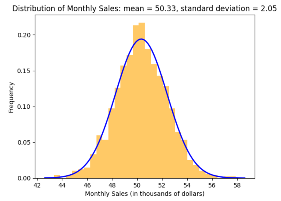
When you observe the histogram and the overlaid curve, you see a bell-shaped, symmetric appearance. This indicates that the sales data follows a normal distribution, meaning:

• Most sales values cluster around the mean (average monthly sales).
• The frequency of sales values decreases symmetrically as you move away from the mean.

1a. Normal Distribution

The normal distribution, also known as the Gaussian distribution, is a continuous probability distribution that is symmetrical around its mean. This means that most of the data points cluster around the central peak, and the data values taper off away from the mean equally in both directions. There are different kinds of normal distributions. For example, the figure below illustrates four different normal distributions that have different means and standard deviations.

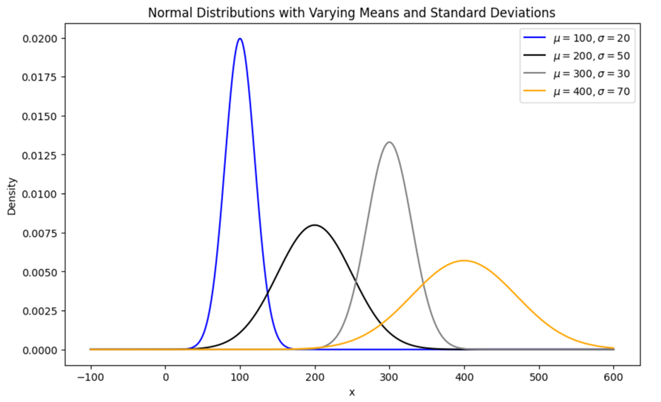
Below are some key characteristics of the normal distribution.

Symmetrical: The bell-shaped curve is symmetrical around the mean. This symmetry indicates that data points are equally likely to occur on either side of the mean.

Mean-Centered: The mean is the center of the distribution. Each curve peaks at its respective mean value, showing where the data is most concentrated.

Variability: The standard deviation determines the spread of the distribution. A larger standard deviation results in a wider, flatter curve, indicating more variability in the data. Conversely, a smaller standard deviation results in a narrower, taller curve, indicating less variability.

Probability: The height of the curve at any given point represents the probability density. Higher peaks indicate a higher likelihood of values near the mean, while the tails show that extreme values are less likely.

Finding Probabilities: To find probabilities for data that follows a normal distribution, you use the density function (the curves that you see drawn in the figure above). To find a probability, you are really finding the area under the curve.

Here’s a simple way to think about it:

• Less Than a Value: To find the probability of getting a value less than a certain number, you look at the area under the curve to the left of that number.
• Greater Than a Value: To find the probability of getting a value greater than a certain number, you look at the area under the curve to the right of that number.
• Between Two Values: To find the probability of getting a value between two numbers, you look at the area under the curve between those two numbers.

Let’s take a look at how you would determine the probability of certain events occurring if your data was normally distributed.

term to know

Normal Distribution

A continuous distribution that is bell-shaped and is symmetric about its mean when the distribution is visualized.

1b. Finding Probabilities Using the Normal Distribution

Let’s look at how you apply and use the normal probability distribution in several real-world business data analytics scenarios.

EXAMPLE

Suppose you are working for a social media company. Your task is to analyze the engagement data (likes, comments, and shares) for a popular influencer’s posts over the past year. The company wants to understand the distribution of engagement and evaluate probabilities to gain insights about future posts. You have been asked to calculate three probabilities for them.

1. This calculates the probability that a post receives 400 or fewer engagements.
2. This calculates the probability that a post receives more than 600 engagements.
3. where X is the number of engagements. This calculates the probability that a post gets between 450 and 550 engagements.

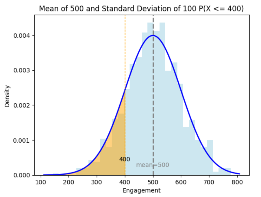
The graph above illustrates the for engagement data of an influencer’s posts. The light blue bars represent the histogram of the engagement data (likes, comments, and shares) for the influencer’s posts. The height of each bar indicates the frequency of posts with a certain level of engagement.

The blue curve is the normal distribution curve, which models the engagement data with a mean of 500 and a standard deviation of 100. It shows the theoretical distribution of engagement levels.

The orange area that is shaded is the region under the normal distribution curve and represents the probability It shows a post's likelihood of receiving less than 400 engagements.

The dashed vertical orange line at 400 engagements marks the threshold. Everything to the left of this line (the orange area) is included in the probability calculation.

The dashed grey vertical line at 500 represents the mean of the number of engagements in the data.

You find the probability that the influencer receives less than 400 engagements is 16%. You will find this probability in the upcoming example. This has practical implications that you can report back to the social media company, including:

1. Engagement Benchmarking.

• Threshold Identification. The 400 engagements mark can be used as a threshold to identify underperforming posts. Since only 16% of posts fall below this threshold, it indicates that posts with fewer than 400 engagements are significantly underperforming compared to the average.

2. Content Strategy.

• Performance Monitoring: Regularly monitor the influencer’s posts to ensure that the majority are performing above this threshold. This can help in maintaining a high standard of content and engagement.
• Feedback and Training: Provide feedback and training to the influencer to help them understand what content types are more likely to engage their audience and avoid those that fall below the 400 engagements mark.

3. Audience Analysis.

• Analyze the posts that fall below the 400 engagements threshold to understand what might not be resonating with the audience. This can provide valuable insights into audience preferences and behavior.
• Segment the audience to identify which groups are less engaged and tailor content specifically to re-engage these segments.

By finding and reporting this one probability, it allows for insights the social media company can use to make data-driven decisions to enhance their content strategy, improve influencer performance, and ultimately increase overall engagement rates.

EXAMPLE

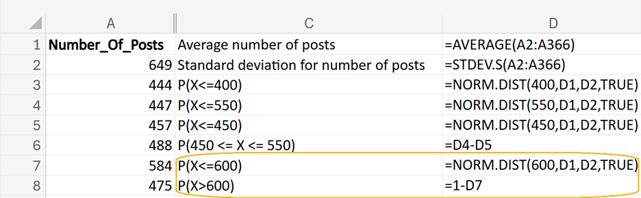
Use Excel to find the probability that a post receives 400 or fewer engagements, In Excel, open the social_media_engagement_posts.xlsx file. The column Number_Of_Posts contains the daily number of different engagement types, such as likes, comments, and shares, for a popular social media influencer for one year.

Perform the following.

1. Enter Average number of posts in cell C1.

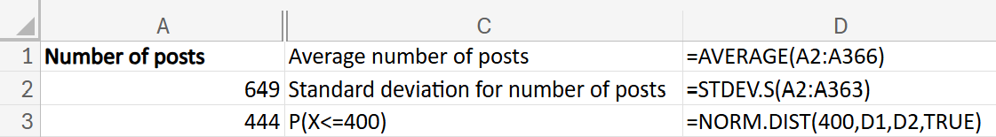
In cell D1, enter the following formula:

=AVERAGE(A2:A365)

2. Enter Standard deviation for number of posts in cell C2.

3. In cell D2, enter the following formula:

=STDEV.S(A2:A366)

4. Enter P(X<=400) in cell C3.

In cell D3, enter the following formula:

=NORM.DIST(400,D1,D2,TRUE)

The NORM.DIST() function calculates probability using the normal distribution function with a specified mean and standard deviation. The function takes several arguments that are described below.

• NORM.DIST(x, mean, standard_dev, cumulative) is the Excel function with four arguments.
  • x: The value for which you want the distribution (in this case, 400 posts).
  • mean (D1): The arithmetic mean of the distribution (in this case, 500).
  • standard_dev (D2): The standard deviation of the distribution (in this case, 100).
  • cumulative: A logical value that determines the form of the function. Use TRUE for the cumulative distribution function. That is, TRUE will return the probability of receiving less than or equal to 400 posts.

The completed Excel worksheet, along with the Excel formulas, is shown in the screenshots below.





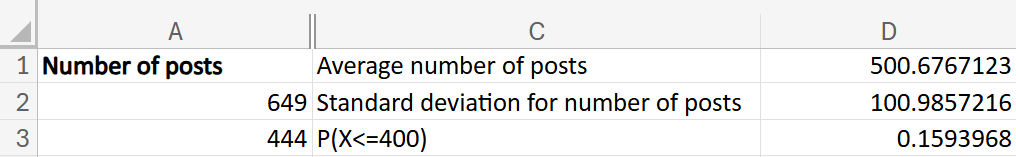
The probability that a post will receive 400 or fewer is 15.94%.

try it

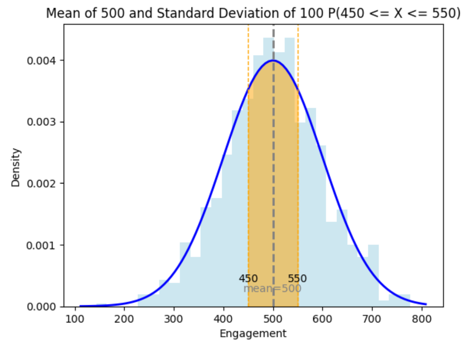
Use Excel to find the probability that a post receives between 450 and 550 engagements, The data is in social_media_engagement_posts.xlsx. The column Number_Of_Posts contains the daily number of different engagement types, such as likes, comments, and shares, for a popular social media influencer for one year.

Answer: 38%

The probability you are trying to find is shown in the orange shaded area below.



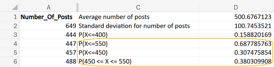
1. Enter P(X<=550) in cell C4.

In cell D4, enter the following formula:

=NORM.DIST(550,D1,D2,TRUE)

2. Enter P(X<=450) in cell C5.

In cell D5, enter the following formula:

=NORM.DIST(450,D1,D2,TRUE)

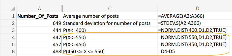
3. Enter P(450<=X<=550) in cell C6.

In cell D6, enter the following formula:

=D4-D5

By subtracting the two probabilities, =NORM.DIST(550, mean, standard_dev, TRUE) - NORM.DIST(450, mean, standard_dev, TRUE), this provides you with the probability that the post receives between 450 and 550 engagements.

The completed Excel worksheet, along with the Excel formulas, is shown in the screenshots below.

think about it

What is a practical interpretation of the probability that a post receives between 450 and 550 engagements that you could share with the social media company?

try it

Use Excel to find the probability that a post receives more than 600 engagements, The data is in social_media_engagement_posts.xlsx. The column Number_Of_Posts contains the daily number of different engagement types, such as likes, comments, and shares, for a popular social media influencer for one year.

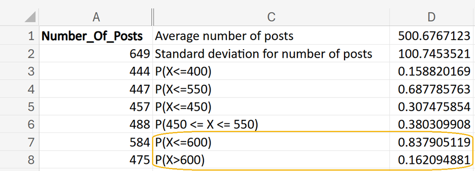
Answer: 16.19%

The probability you are trying to find is shown in the orange shaded area below.



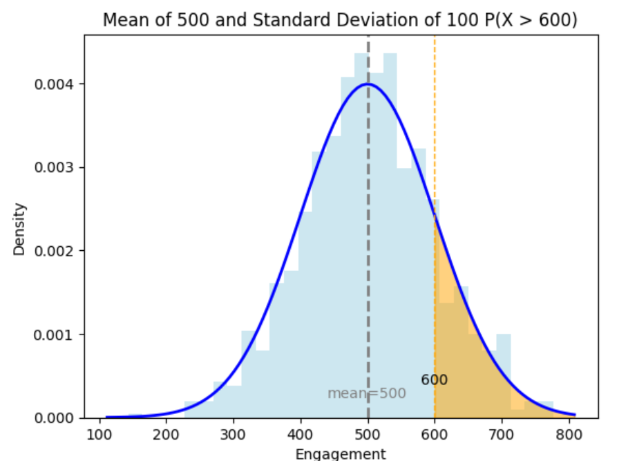
1. Enter P(X<=600) in cell C7.

In cell D7, enter the following formula:

=NORM.DIST(600,D1,D2,TRUE)

2. Enter P(X>600) in cell C8.

In cell D8, enter the following formula:

=1 - NORM.DIST(600,D1,D2,TRUE)

The reason you subtract the cumulative probability from 1 is that you are essentially finding the complement of cumulative probability. The cumulative probability, gives you the probability that a value is less than or equal to 600.

To find the probability that a value is greater than 600, you need to consider the remaining portion of the distribution. Since the total probability for any distribution is 1 (or 100%), you subtract the cumulative probability from 1.

The completed Excel worksheet, along with the Excel formulas, is shown in the screenshots below.

think about it

What is a practical interpretation of the probability that a post receives more than 600 engagements that you could share with the social media company?

did you know

In the context of the normal distribution, the is the same as the because the distribution is continuous.

In a continuous distribution like the normal distribution, there are an infinite number of possible values within any range. This means that the probability of any single, exact value (like exactly 600) is essentially zero.

When you calculate probabilities for data that follows a normal distribution, you are looking at the area under the curve. Since the area at a single point is zero, including or excluding that point does not change the total area.

So, when you calculate the you are finding the area under the curve to the left of 600. And when you calculate you are also finding the area under the curve to the left of 600.

This same logic is true for greater than probabilities and between probabilities when using the normal distribution.

Below is a table that can be used as a reference for when and how to use the NORM.DIST() Excel functions.

Let’s get some more practice! Below is another exercise that will give you more experience with finding probabilities from a normal distribution in Excel.

try it

You are a data analyst at a digital marketing agency. Your task is to analyze the website traffic data for a client’s website over the past year. The company wants to understand the distribution of traffic and find probabilities of achieving certain traffic thresholds.

You create a histogram of the number of page views, overlay a normal distribution over the histogram, and observe the data is normally distributed.



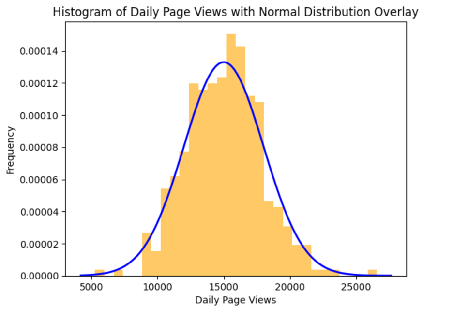
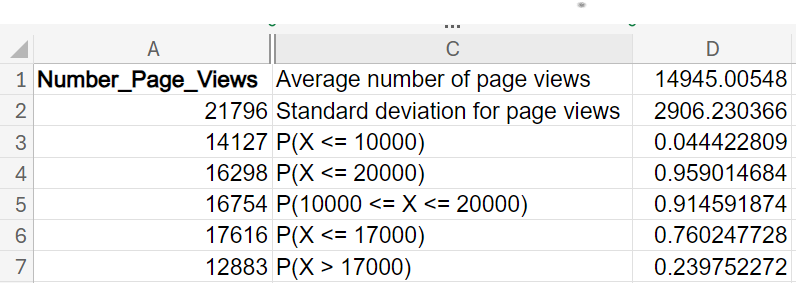
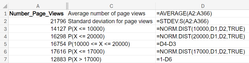
Find the following probabilities using the appropriate Excel function. The data is in the Excel file website_traffic.xlsx, where each row represents the number of page views for the client’s website. Provide a practical interpretation of the probability in the context of the problem.

What is the probability that the number of page views in a given day is less than 10,000?

4.44%. On approximately 4% of the days, the website is expected to receive fewer than 10,000 page views. This information can help the company understand the frequency of lower traffic days and potentially identify patterns or factors contributing to these lower traffic periods.

What is the probability that the number of page views in a given day is between 10,000 and 20,000?

91.46%. This probability means that on most days (approximately 91% of the time), the website’s daily traffic falls within this range. This high probability indicates that the website consistently attracts a substantial amount of traffic, suggesting stability and reliability in its performance. Knowing that the website frequently receives between 10,000 and 20,000 views can help in planning marketing campaigns, as you can expect a certain level of engagement.

What is the probability that the number of page views in a given day exceeds 17,000?

23.98%. On approximately 24% of the days, the website experiences high traffic, with more than 17,000 page views. Identifying the factors that contribute to these high-traffic days can help in replicating successful strategies.

Reference Excel Calculations.

The completed Excel worksheet, along with the Excel formulas, is shown in the screenshots below.

watch

Follow along with the video to help the company understand the distribution of traffic and find probabilities of achieving certain traffic thresholds.