Table of Contents |
In your previous tutorials, you learned how to build a simple linear regression model in Python to predict the amount of donations based on the number of social media shares a donation campaign receives. This was a great starting point to understand the relationship between two variables.
Now, let’s take it a step further and explore multiple linear regression. While simple linear regression involves one predictor variable, multiple linear regression allows us to include multiple explanatory variables to better understand and predict the response variable.
Imagine you are still working with the non-profit organization, but now you have additional data that might predict donation amounts. For example, besides the number of social media shares, you also have information on the amount spent on marketing and the number of email subscribers. By incorporating these additional explanatory variables, you can build a more comprehensive model that captures the combined effect of all these factors on the donation amounts.
By the end of this tutorial, you will be equipped with the skills to build and interpret multiple linear regression models, enabling you to make more informed decisions based on a broader set of data.
Let’s get started on this exciting journey into multiple linear regression!
In previous tutorials, you learned about simple linear regression, which helps you understand the relationship between a response and an explanatory variable. For example, you used the number of social media shares to predict the amount of donations a campaign receives. The equation for simple linear regression looks like this:

 is the predicted value of the response variable
  is the y-intercept
  is the slope
  is still the predicted value of the response variable (amount of donation).
 and
and  are the explanatory variables (number of social media shares, amount spent on marketing, and number of email subscribers, respectively). is the y-intercept.
 and
and  are the coefficients that show the impact of the explanatory variables on the response variable.
 For example, using multiple linear regression, you can predict the amount of donations more accurately by considering not just social media shares but also how much money was spent on marketing and how many email subscribers the fundraising campaign has.
This method is powerful because it gives you a more complete picture and helps you make better decisions based on multiple pieces of information.
The general multiple regression for p explanatory variables is given by:
 number of social media shares. amount spent on marketing.
  Lighter colors mean fewer subscribers, and darker colors mean more subscribers.
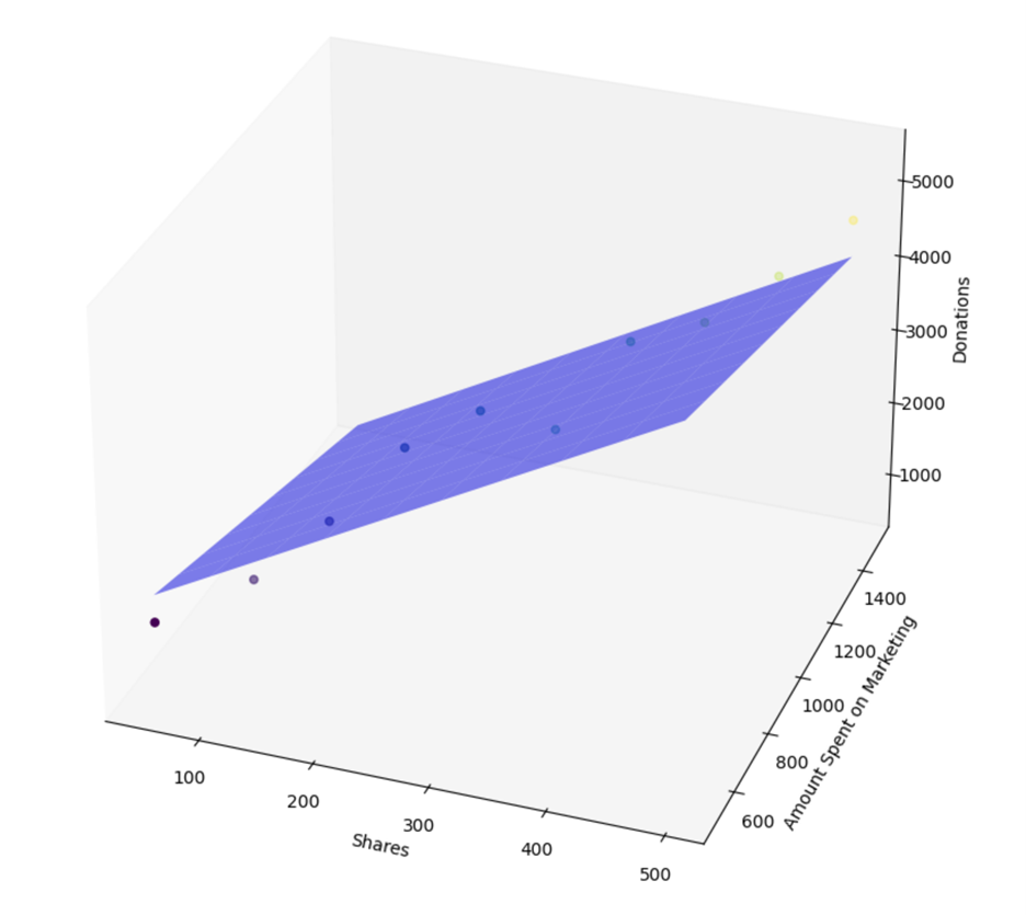
Now, you are ready to build a multiple linear regression model for the amount of donations the non-profit will receive, based on the number of social media shares a campaign receives, the amount of marketing spent on the fundraising campaign, and the number of email subscribers there are for each campaign.
The data is contained in an Excel file stored on GitHub named:
https://raw.githubusercontent.com/sophiaAcademics/BDA_Excel/main/StudentData/Tutorials/Unit5/5.1.4/donations_multiple_regression.xlsx
The data has four variables, as described below:


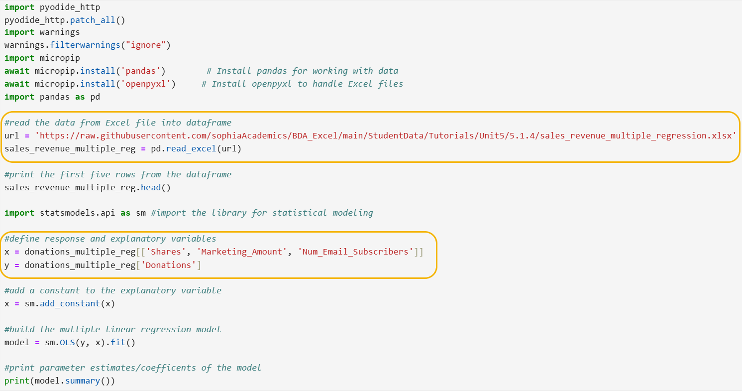
The code below imports pandas, imports an Excel file from a URL, creates a pandas DataFrame, and displays the first five rows of the DataFrame.
The summary of the regression model is provided below.
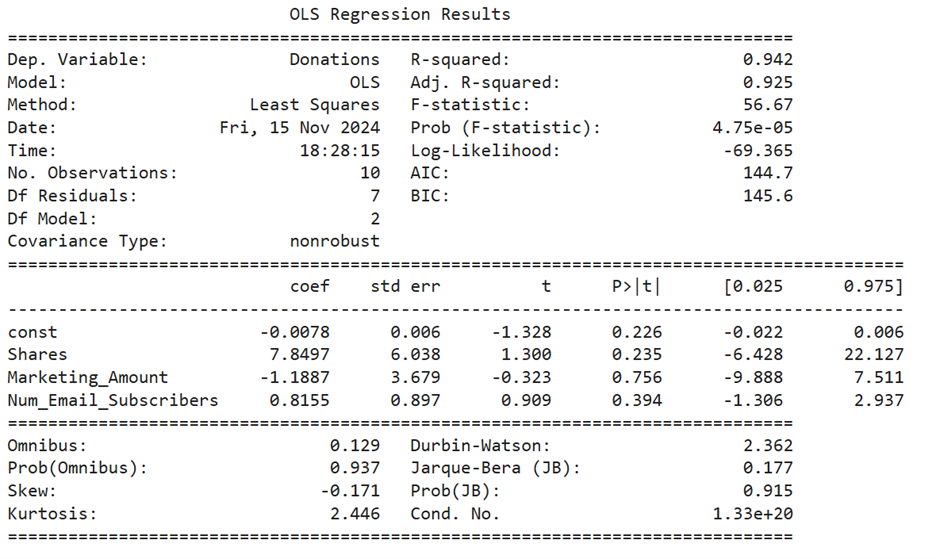
Let's explore the multiple linear regression model output below, where key areas have been highlighted to guide your interpretation and understanding of the model's results.
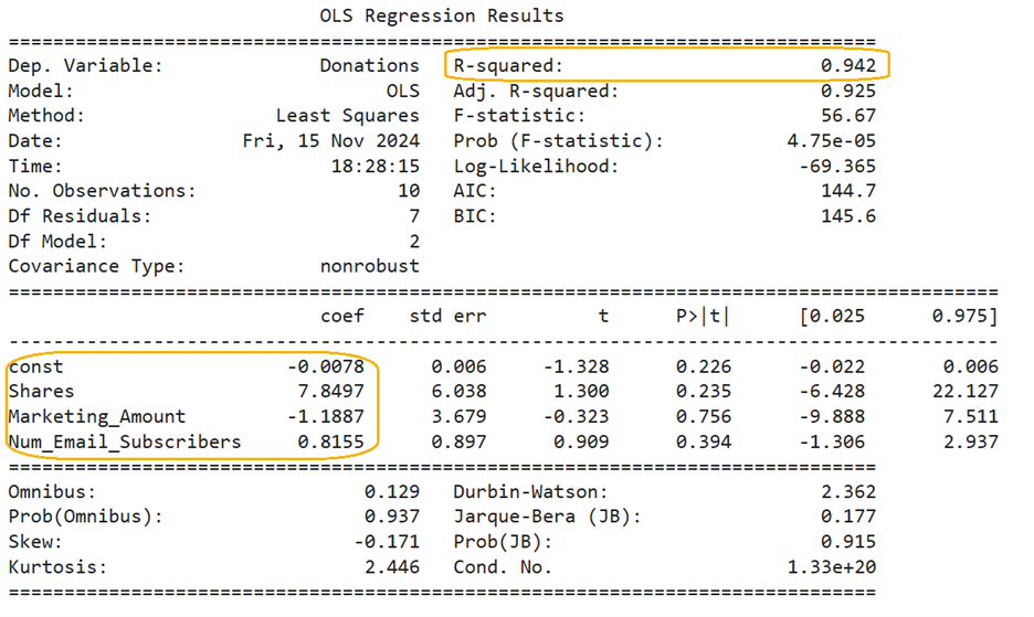
1.  (Coefficient of Determination)
In a previous tutorial, when you used just the number of social media shares to predict the donation amount, the  value was 94.1%. This means that 94.1% of the variation in donation amounts could be explained by social media shares alone.
Now, after adding marketing spend and the number of email subscribers to the model, the value increased slightly to 94.2%. This tells you several things:
suggests that most of the predictive power comes from the number of social media shares, and the other explanatory variables (marketing spend and email subscribers) have a much smaller impact. In summary, while adding more variables can sometimes improve a model, in this case, the number of social media shares is already doing most of the work in predicting donation amounts. You will soon learn how to test if the additional variables are truly useful predictors.
2. coef column
in the regression equation  in the regression equation The value of is 7.85.
 in the regression equation The value of is -1.19. in the regression equation The value of is 0.82.
Interpreting the Model:
Each coefficient in the model quantifies the relationship between the corresponding explanatory variable and the response variable while accounting for the effects of the other variables in the model. This allows you to understand the individual impact of each explanatory variable on the predicted amount of donation. For example:
 This coefficient (7.85) indicates the change in the predicted amount of donation for each additional social media share, holding all other variables constant. Specifically, for each additional social media share, the predicted amount of donation increases by $7.85.
  This coefficient (-1.19) shows the change in the predicted amount of donation for each additional unit of money (dollar in this case) spent on marketing, holding all other variables constant. Here, for each additional dollar spent on marketing, the predicted amount of donation decreases by $1.19. This negative coefficient might suggest that beyond a certain point, additional marketing expenditure does not translate into higher donations, or it could indicate inefficiencies in the marketing strategy.
  This coefficient (0.82) represents the change in the predicted amount of donation for each additional email subscriber, holding all other variables constant. Thus, for each additional email subscriber, the predicted amount of donation increases by $0.82.
 Now, it is your turn to build and interpret a multiple linear regression model in Python!
value. value to the value for the simple linear regression that was found in a previous tutorial to predict sales revenue using marketing spend. What does the increase/decrease in the value for the multiple linear regression tell you? 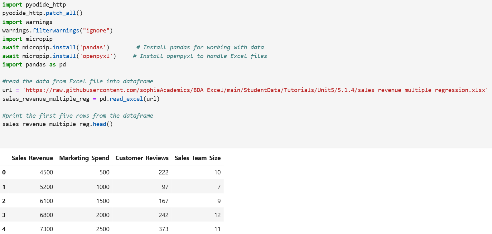
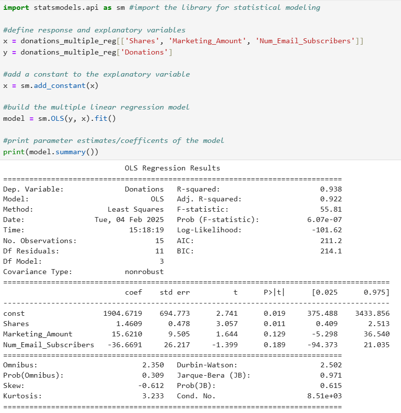 value from the regression output is 99.6%. 99.6% of the amount of variability in sales revenue can be explained using the amount spent on marketing, the number of customer reviews posted on the website, and the number of team members on the sales team.
value was 99.4%. This means that marketing spend alone is already a very strong predictor of sales revenue, explaining 99.4% of the variability.
value from the regression output is 99.6%. 99.6% of the amount of variability in sales revenue can be explained using the amount spent on marketing, the number of customer reviews posted on the website, and the number of team members on the sales team.
value was 99.4%. This means that marketing spend alone is already a very strong predictor of sales revenue, explaining 99.4% of the variability.

 This coefficient indicates that for every additional dollar spent on marketing, the predicted sales revenue increases by $1.24, holding the number of customer reviews and the size of the sales team constant. This suggests that marketing spend has a positive impact on sales revenue.
  This coefficient shows that for each additional customer review, the predicted sales revenue increases by $0.33, holding marketing spend and sales team size constant. This means that more customer reviews are associated with higher sales revenue, although the impact is smaller compared to marketing spend.
  This coefficient represents the change in predicted sales revenue for each additional member of the sales team, holding marketing spend and customer reviews constant. Specifically, for each additional sales team member, the predicted sales revenue increases by $20.10. This indicates that having a larger sales team greatly enhances the predicted sales revenue. (coefficient of determination) and the values of the coefficients from the model. measures how well the explanatory variables account for the variability in the response variable, while the coefficients quantify the relationship between each explanatory variable and the response variable. Both interpretability methods are important in a multiple linear regression because they provide a comprehensive understanding of the model's performance and the individual contributions of each explanatory variable, enabling more informed decision-making.
Source: THIS TUTORIAL WAS AUTHORED BY SOPHIA LEARNING. PLEASE SEE OUR TERMS OF USE.