In this lesson, you will learn about the standard normal distribution and how to use the distribution to find probabilities for business analytics scenarios. Specifically, this lesson will cover:
-
This lesson builds on key concepts from an Introduction to Statistics course. Specifically, this tutorial assumes familiarity with the foundational ideas of normal distribution and z-scores.
1. Introduction to the Standard Normal Distribution
Imagine you are analyzing the number of smartphones sold by a large telecommunications company across two sales regions for the last month. You have collected data and found that the number of smartphones sold in each region follows a normal distribution. Here are the statistics:
-
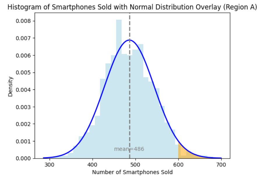
Region A: The average (mean) number of smartphones sold is 486, with a standard deviation of 58.
-
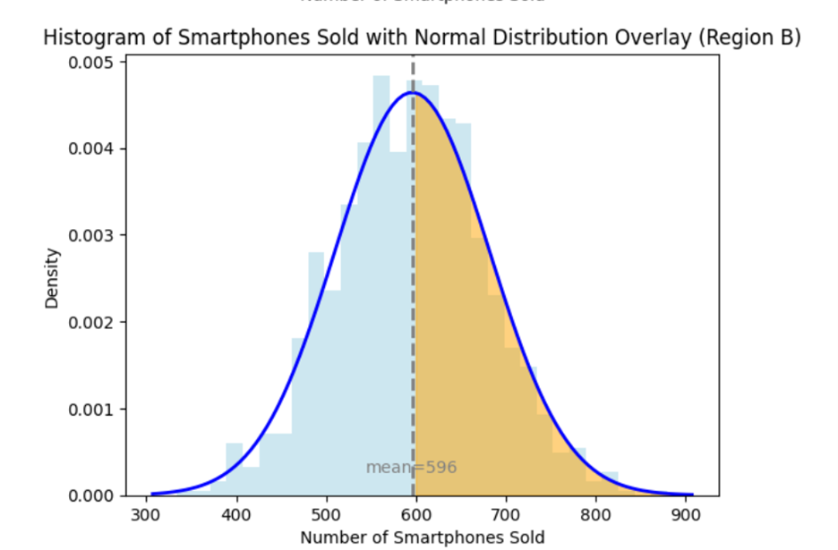
Region B: The average (mean) number of smartphones sold is 596, with a standard deviation of 86.
The company has set a sales goal of 600 smartphones for each region. Your goal is to find out the probability that each region will achieve this target.
You graph the histogram of the number of smartphones each region has sold and overlay a normal probability distribution on the histogram. You observe that both distributions follow a normal distribution with different means and standard deviations. The two graphs below show the distribution of the number of smartphones for both regions, where the orange shaded area visually shows the probability of each region achieving the sales goal (more than 600 units sold).
When you look at the raw distributions of the number of smartphones sold in Regions A and B, you observe that the sales target of 600 is positioned differently relative to each region’s mean and standard deviation.
-
Region A: The mean is 486, and the standard deviation is 58. The target of 600 units is far from the mean, making it an extreme value.
-
Region B: The mean is 596, and the standard deviation is 86. The target of 600 units is much closer to the mean, making it a more typical value.
The means and standard deviations are different for each region. This means the center of data and spread of the data are not aligned in the graphs above, making it visually challenging to compare how far 600 units is from the mean in each region. In Region A, 600 units is in the far-right tail of the distribution, indicating a low probability of achieving this target. In Region B, 600 units is near the center, indicating a higher probability. Without
standardizing the data, these differences in tail positions make it hard to directly compare the probabilities. By standardizing the data, you can fairly compare the probabilities of achieving the sales target in both regions.
-
- Standardization
- The process of converting data so that all the values have the same measurement scale.
1a. Standard Normal Distribution
The standard normal distribution is a special type of normal distribution that has some special properties:
- Mean is 0
- Standard deviation is 1
The standard normal distribution helps you compare different normal distributions. In simpler terms, the standard normal distribution is like a universal ruler that helps you measure and compare different sets of data on the same scale. The standard normal distribution is made up of
z-scores, which standardize data points and allow you to compare and interpret data points on a common scale. Z-scores allow you to compare data points from different distributions, even if they have different means and standard deviations.
A z-score informs you of how far above or below a data point is from its mean.
The graph below shows you the standard normal distribution.
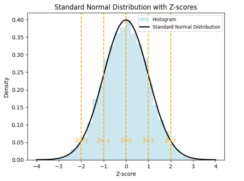
The table describes what each z-score means in the context of the standard normal distribution.
|
z-score
|
Description
|
|
-2
|
The data point is two standard deviations below the mean.
|
|
-1
|
The data point is one standard deviation below the mean.
|
|
0
|
The data point is exactly at the mean.
|
|
1
|
The data point is one standard deviation above the mean.
|
|
2
|
The data point is two standard deviations above the mean.
|
The z-scores allow you to convert a data point to the standard normal distribution by using the formula:

Where
X is the specific data point you are interested in converting to the standard normal distribution,

is the sample average of the data points, and
s is the sample standard deviation of the data points in the data.
-
EXAMPLE
Referring to the number of smartphones sold in Regions A and B, calculate and interpret the z-score for the sales target of 600 smartphone units for both regions.
Region A: 

and the specific data point is 600.

The z-score is

A z-score of 1.97 means that the sales target of 600 units is 1.97 standard deviations above the mean of 486.
Region B: 

and the specific data point is 600.

The z-score is 0.05. A z-score of 0.05 means that the sales target of 600 units is 0.05 standard deviations above the mean of 596.
Standardizing the data allows you to compare the sales performance of different regions on a common scale, despite their differing means and standard deviations. Here’s a summary of how this process provides valuable insights:
-
Fair Comparison: By converting the sales target to a z-score, you can directly compare the performance of Region A and Region B, even though their average units and variability differ. This helps in understanding how exceptional or common a sales figure is in each region.
-
Probability Calculation: Standardizing enables you to use the standard normal distribution to calculate the probability of achieving the sales target. This reveals how likely each region is to meet or exceed the goal, providing a clear picture of their performance.
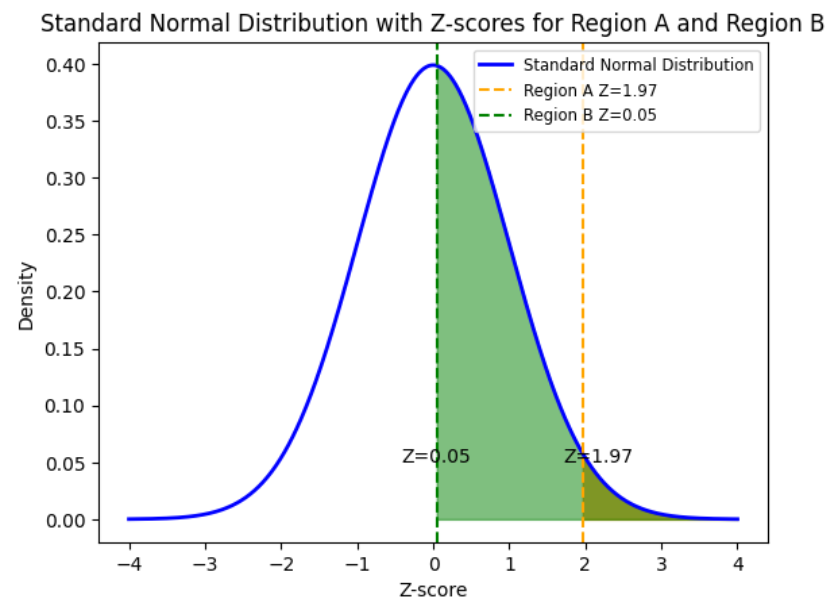
The graph below shows the standardized distributions (z-scores) for both regions overlaid on each other. By converting the data to z-scores, you can see how far the sales target is from the mean in terms of standard deviations. Region A with a z-score of 1.97 indicates that the sales target value of 600 is 1.97 standard deviations above the mean of the sales data. In other words, it is significantly higher than the average sales value. Region B with a z-score of 0.05 means the sales target of 600 is 0.05 standard deviations above the mean. This suggests that it is slightly above average, but not significantly so. The graph visually shows you that Region A, with a higher z-score, means a more ambitious or challenging sales target, while a lower z-score suggests Region B is a more achievable or less aggressive target. This standardization allows for a fair comparison of the probabilities.
In the next section, you will obtain some hands-on practice using Excel to calculate these probabilities from the standard normal distribution.
-
- Standard Normal Distribution
- A normal distribution that has a mean of 0 and a standard deviation of 1.
- z-score
- A statistical measurement that defines a data point’s position relative to its mean.
1b. Finding Probabilities Using the Standard Normal Distribution
Now that the basics of the standard normal distribution and z-scores have been covered, let’s return to the example of smartphone sales and use the probabilities to provide insight to the telecommunications company. Then, you will use Excel to compute the probabilities.
-
EXAMPLE
Recall you are analyzing the number of smartphones sold by a large telecommunications company across two of their sales regions for the last month. You graph the distribution of the number of smartphones (units) for each region and find that the data is normally distributed.
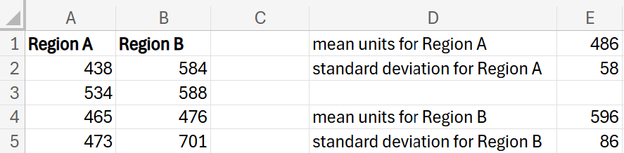
In Excel, you compute the mean and standard deviation of the number of smartphone units sold and find that the regions have different means and standard deviations. From your data in Excel, you find that the mean number of smartphones sold in Region A is 486 with a standard deviation of 58. In Region B, you find that the mean number of smartphones sold is 596 with a standard deviation of 86.
The company has recently set a sales goal that it wants each region to sell at least 600 smartphones each month. The company has asked you to find the probability that each region achieves this target sales goal; that is, you need to find the probability that each region will sell more than 600 smartphones.
You recognize that standardizing the sales data will allow for a fair comparison of the probabilities between the two regions. Despite the sales target of 600 units being the same, the probability of achieving this target differs significantly between the two regions due to their different means and standard deviations.
- Region A has a lower mean and smaller standard deviation, making sales of 600 units much more exceptional, which will result in a higher z-score and lower probability.
- Region B has a higher mean and larger standard deviation, making sales of 600 units less exceptional, which will result in a lower z-score and higher probability.
You standardize the data and find the probabilities using the standard normal distribution. You determine the following probabilities:
- Region A: The probability that Region A will sell more than 600 smartphones in one month is 2.47%.
- Region B: The probability that Region B will sell more than 600 smartphones in one month is 48.15%.
Practical Interpretations:
Below are some practical interpretations of the probabilities you can provide to the telecommunications company.
Region A (2.47%): This very low probability indicates that it is highly unlikely for sales in Region A to exceed 600 units. Given the mean number of 486 units and a standard deviation of 58 units, a figure of 600 units is quite far from the average. This suggests that achieving such a high number of units in Region A would be an exceptional event, occurring only about 2.47% of the time.
Region B (48.15%): This higher probability indicates a much more realistic chance of the number of smartphones exceeding 600 units in Region B. With a mean number of 596 units and a standard deviation of 86 units, a figure of 600 units is close to the average. This means that selling 600 units is relatively common in Region A, occurring almost 50% of the time (48.15%).
Insights:
Based on the probabilities you have calculated, below are some insights the company can gain:
Region A (2.47%):
-
Sales Strategy Reevaluation: The very low probability suggests that the current sales strategies in Region A may not be effective enough to meet the target. The company might need to reevaluate and enhance its marketing and sales tactics in this region.
-
Resource Allocation: Given the low likelihood of achieving the target, it might be beneficial to allocate additional resources, such as more sales personnel or an increased marketing budget, to boost sales in Region A.
-
Product and Market Analysis: Investigate if there are specific factors in Region A, such as market saturation or competition, that are hindering sales. Understanding these factors can help in devising more targeted strategies.
Region B (48.15%):
-
Optimizing Sales Efforts: With a nearly 50% chance of meeting the target, Region B is performing relatively well. The company can focus on fine-tuning its existing strategies to push the probability even higher.
-
Benchmarking Best Practices: Analyze what is working well in Region B and see if those practices can be adapted and implemented in Region A to improve its performance.
-
Market Expansion: Given the higher probability of success, Region B might be a good candidate for market expansion efforts. The company could explore new customer segments or geographic areas within this region to further increase sales.
Being able to interpret and describe how the probabilities from the standard normal distribution can be used in the context of the business analytics problem is beneficial in a couple of ways.
-
Identifying Challenges and Opportunities: The probabilities highlight regions where meeting the sales target is highly unlikely (Region A) versus those where it is more achievable (Region B). This helps in identifying where to focus efforts and resources to improve sales.
-
Strategic Insights: Understanding the standardized probabilities allows the company to tailor strategies for each region. For instance, Region A might need more aggressive marketing or sales support, while Region B could benefit from optimizing existing strategies.
-
Using the number of smartphones that each region has sold in the last 30 days from the previous example, use Excel to find the probability, for both Region A and Region B, that each region sells more than 600 smartphones.
Using the data in the
smartphone_units.xlsx Excel file, perform the following:
1. In cell D1, enter
mean units for Region A.
In cell E1, enter the following formula:
=ROUND(AVERAGE(A2:A31),0)
Using the ROUND() function with an argument of 0, so that you will not receive an average number of smartphones with any decimal points, is a practical consideration since you would never deal with the fractional form of a smartphone.
2. In cell D2, enter
standard deviation for Region A.
In cell E2, enter the formula:
=ROUND(STDEV.S(A2:A31),0)
3. In cell D3, enter
sales target.
In cell E3, enter the value 600.
4. In cell D4, enter
z-score for sales target.
In cell E4, enter the formula:
=(E3-E1)/E2
This formula standardizes the value for 600.
5. In cell D5, enter
P(z < 1.97).
In cell E5, enter the formula:
=NORM.S.DIST(E4,TRUE)
NORM.S.DIST() works in a similar manner to NORM.DIST() from the last tutorial, except now you are finding probabilities from the standard normal distribution (mean of 0 and standard deviation of 1) and not a specific normal distribution with a certain mean and standard deviation.
NORM.S.DIST(z, cumulative) is the Excel function with two arguments. The arguments are described below.
- The z-score (number of standard deviations from the mean) for which you want the distribution.
- cumulative: A logical value that determines the form of the function. Use TRUE for the cumulative distribution function. That is, TRUE will return the probability of obtaining less than z standard deviations.
6. In cell D6, enter
P(z > 1.97).
In cell E6, enter the formula:
=1-E5
In a similar way that you found the “greater than” probabilities by using the rule of complements, you will apply the same logic in the standard normal distribution. The total area under the standard normal distribution curve is 1, representing the total probability. This means that

If you want to find

you are interested in the area to the right of 1.97. Since the total area under the curve is 1, the area to the right of 1.97 is simply the complement of the area to the left of 1.97.
7. Repeat these steps for Region B.
The completed Excel worksheet, along with the Excel formulas, is shown in the screenshots below.
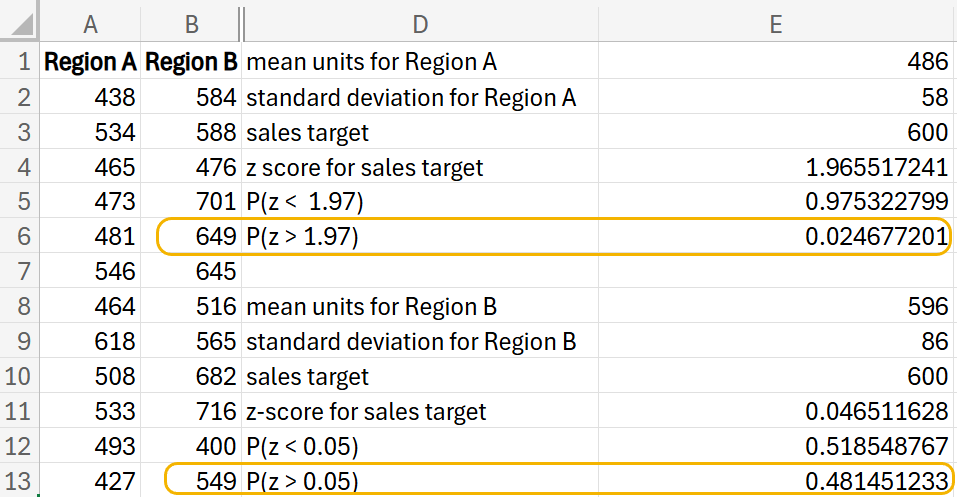
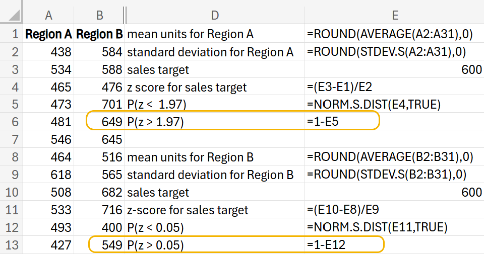
You should obtain the probability for Region A is 2.47% and the probability for Region B is 48.15%.
8. Check your work to ensure you find these same probabilities.
The next problem provides you with more practice computing probabilities from a standard normal distribution in Excel.
-
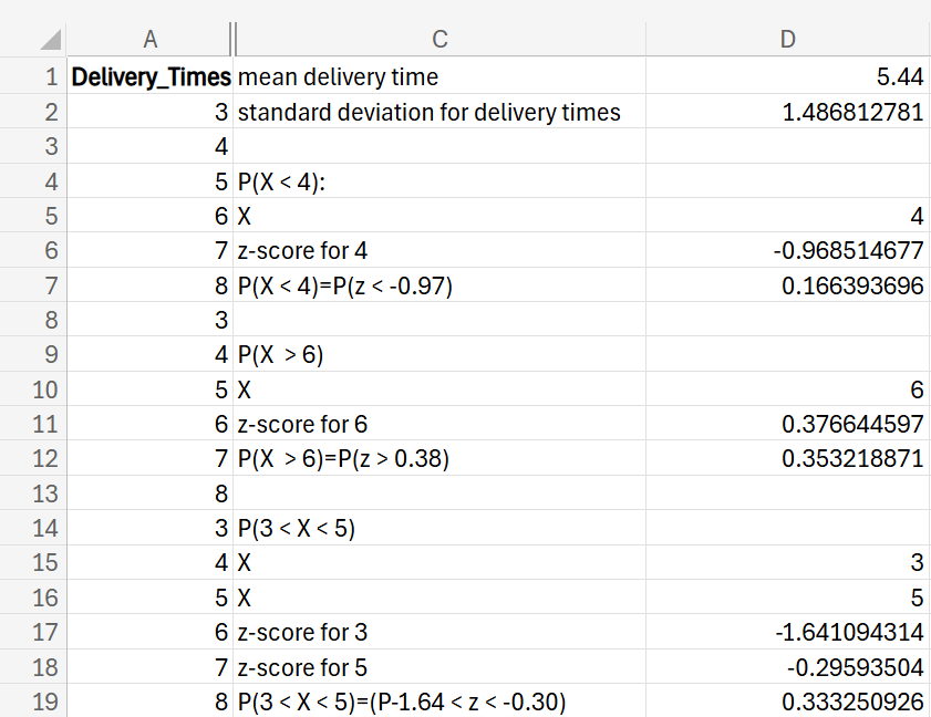
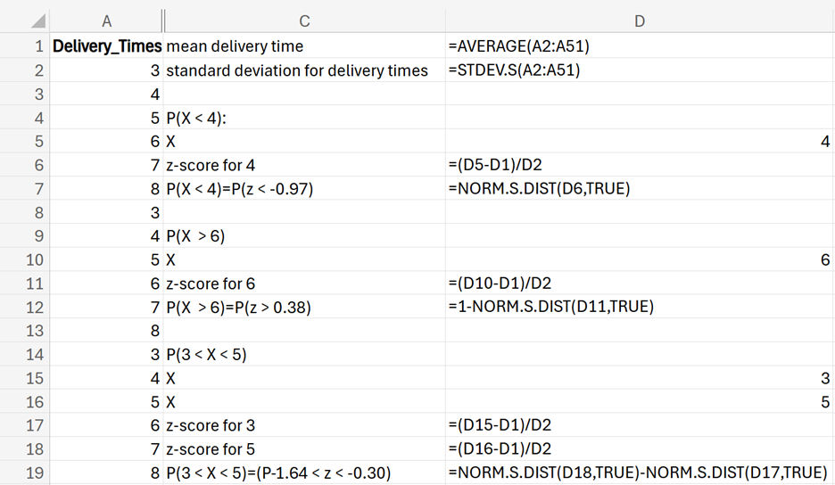
An online retail company wants to analyze its delivery times to ensure customer satisfaction. The company has collected data on delivery times (in days) for their last 50 deliveries. You can presume the delivery times follow a normal distribution.
Using the data in the
delivery_times.xlsx Excel file, use the NORM.S.DIST() Excel function to find the following probabilities.
-
Check out this video about computing probabilities from a standard normal distribution.
-
Why did you use the standard normal distribution for the previous Try It problem instead of just using the normal distribution?
There are several reasons why you would use the standard normal distribution, such as:
By converting data points to z-scores, it standardizes the data points, making it easier to compare and interpret data from different normal distributions. Without standardization, you would need to change the mean and standard deviation values in the NORM.DIST() Excel function.
The standard normal distribution serves as a universal reference. Once data is converted to z-scores, you can use a single Excel function, NORM.S.DIST(), to find probabilities, regardless of the original distribution’s mean and standard deviation.
In this lesson, you explored the standard normal distribution, which is a special normal distribution with a mean of 0 and a standard deviation of 1. The standard normal distribution helps compare different normal distributions. The standard normal distribution is made up of values known as z-scores, which standardize data points and allow you to compare and interpret data points on a common measurement scale. When you standardize data, the data is converted to a scale such that all the data points have the same mean and standard deviation (mean of 0 and standard deviation of 1). This makes it easier to compare different datasets and draw conclusions without needing separate tables for each specific normal distribution.
Converting your data to z-scores and finding probabilities using the z-scores from a standard normal distribution makes for a fairer comparison when comparing two different normal distributions. You found probabilities from a standard normal distribution to provide a deeper understanding of the sales of smartphones in two different regions for a telecommunications company. Using probabilities from the standard normal distribution, the company fairly compared smartphone sales between two regions with different average sales.