Table of Contents |
When you are analyzing data in business, it is important to understand that the data you work with often comes from samples, not the entire population. This means there can be differences between the sample data and the actual population data, which is known as sampling error. These errors can affect the accuracy of your analysis and the decisions you make based on that analysis.
Suppose you are trying to figure out the average amount of money people spend at a store. If you randomly select 10 customers and calculate their average amount spent, the sample mean might differ significantly from the true average amount of money spent by all customers at the store. Asking a small group of people about their spending habits might not perfectly represent everyone who shops there. This difference is a sampling error. If you increase the sample size to 100 customers, the sample mean is likely to be closer to the true population mean. The larger and more diverse your sample, the more likely it is to accurately reflect the whole population, reducing the impact of sampling errors.
Suppose you are analyzing the average amount of money customers spend at a store. Let’s simulate a population of customer spending amounts and draw samples of different sizes to visualize how the sample mean varies and how the standard error changes.
Presume you know that the average amount spent by all customers is $500 and the standard deviation among all the customer spending amounts is $100. That is,  and
and 
You construct two sampling distributions of  The first is 1,000 samples with a sample size of 30, and the second is 1,000 samples with a sample size of 300. You construct two histograms for each sampling distribution and overlay a normal distribution over the histogram, as shown below.
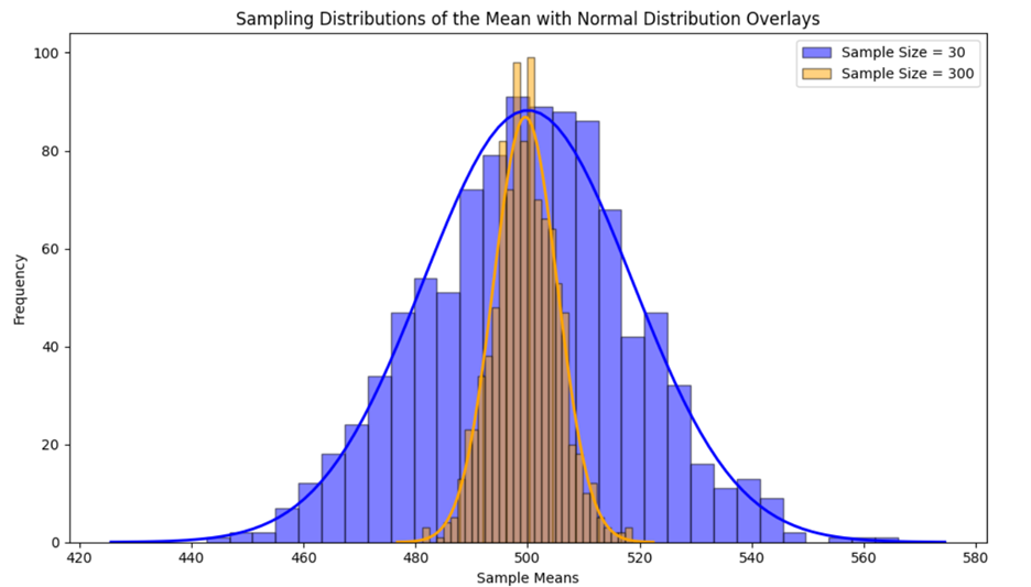
The histogram for the smaller sample size (30) shows more spread and variability in the sample means compared to the histogram for the larger sample size (300). This indicates that the sample means from smaller samples are more dispersed around the population mean.
The histogram for the larger sample size (300) is smoother and more bell-shaped, closely approximating a normal distribution. This is due to the Central Limit Theorem, which states that the sampling distribution of  will be approximately normal for large sample sizes.
The standard error, which measures the variability of the sampling distribution of , is smaller for the larger sample size (300). This is evident from the narrower spread of the histogram. A smaller standard error means that the sample mean is a more precise estimate of the population mean. Standard error is a metric used to measure sampling error.
You can calculate the standard error for each distribution to numerically confirm that the amount of variability in the sampling distribution of with a sample size of 300 is less than the amount of variability in the sampling distribution of with a sample size of 30.
| Sample Size | Number of Samples | Standard Error |
|---|---|---|
| 30 | 1000 |

|
| 300 | 1000 |

|
In summary, the standard error provides a measure of how much the sample mean (or other statistic) is expected to vary from the true population mean due to sampling error. A smaller standard error indicates that the sample mean is likely to be closer to the population mean, while a larger standard error suggests more variability and thus more sampling error. You can think of standard error as a measure of accuracy of which a sample represents a population.
is a more accurate and precise point estimate of μ.
is a less accurate and less precise point estimate of μ.
The concepts of sampling error, standard error, and the Central Limit Theorem apply equally to both sample means and sample proportions. Whether estimating a population mean or a population proportion, the variability of sample estimates, the shape of their sampling distributions, and the precision of these estimates (as measured by the standard error) follow the same rules. This consistency ensures that these foundational statistical concepts can be reliably applied across different types of data, supporting accurate analytical outcomes. Let’s now explore the sampling error for proportions motivated by an example.
Suppose you are a business analyst at an online retail company. You want to estimate the proportion of customers who make a purchase after visiting the website. Instead of surveying every visitor, you take samples of visitors to estimate this proportion.
Presume you know that 40% of all customers make a purchase after visiting the website, that is, you know the true population proportion p.
You construct two sampling distributions of  The first is 1,000 samples with a sample size of 50, and the second is 1,000 samples with a sample size of 500. You construct two histograms for each sampling distribution and overlay a normal distribution over the histogram, as shown below.
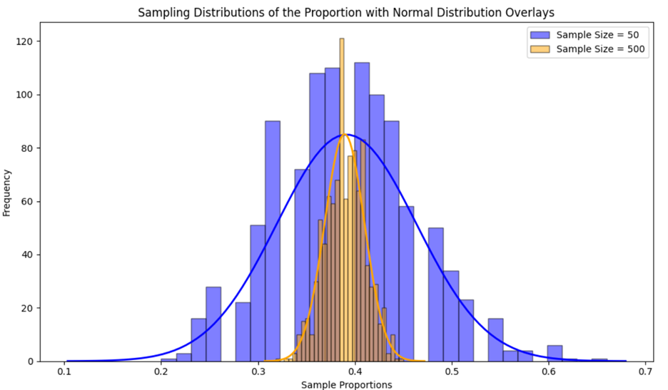
The histogram for the smaller sample size (50) shows more spread and variability in the sample proportions compared to the histogram for the larger sample size (500). This indicates that the sample proportions from smaller samples are more dispersed around the population proportion.
The histogram for the larger sample size (500) is smoother and more bell-shaped, closely approximating a normal distribution. This is due to the Central Limit Theorem, which states that the sampling distribution of  will be approximately normal for large sample sizes.
The standard error, which measures the variability of the sampling distribution of  is smaller for the larger sample size (500). This is evident from the narrower spread of the histogram. A smaller standard error means that the sample proportion is a more precise estimate of the population proportion.
You can calculate the standard error for each distribution to numerically confirm that the variability in the sampling distribution of with a sample size of 500 is smaller than the variability in the sampling distribution of with a sample size of 50. This provides validation that larger sample sizes result in less variability in the sampling distribution.
| Sample Size | Number of Samples | Standard Error |
|---|---|---|
| 50 | 1000 |

|
| 500 | 1000 |

|
is a more accurate and precise point estimate of p.
is a less accurate and less precise point estimate of p.
Source: THIS TUTORIAL WAS AUTHORED BY SOPHIA LEARNING. PLEASE SEE OUR TERMS OF USE.