Table of Contents |
A sampling distribution is a way to understand how a statistic (like an average) from a sample can vary. Imagine you want to know the average amount of money customers spend at a store. Instead of asking every customer, you take several small samples and calculate the average for each sample. The collection of these averages forms a sampling distribution.
Sampling distributions help us understand the variability of our sample statistics. This is important because it allows businesses to make predictions and decisions based on sample data, rather than needing to survey an entire population.
Let’s say a company wants to know the average amount of time customers spend on their website. Instead of tracking every single visitor, they take multiple samples of 100 visitors each and calculate the average time spent for each sample. These averages might be slightly different, but together they form a sampling distribution.
Imagine you take 10 different samples of 100 visitors each and calculate the average time spent on the website for each sample. You might get averages like 5 minutes, 5.2 minutes, 4.8 minutes, etc. If you plot these averages on a graph, you’ll see a distribution of these sample averages. This is your sampling distribution. The histogram below shows a sampling distribution of the average time spent on a website using 10 different samples of 100 visitors each.
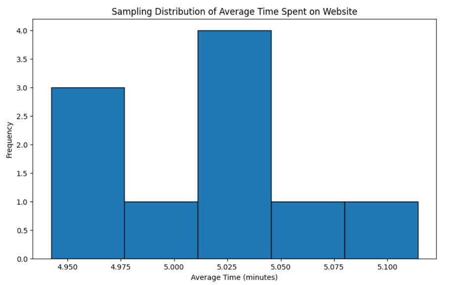
Understanding sampling distributions helps businesses make better decisions. For example, if the sampling distribution shows that most sample averages are around 5 minutes, the company can be confident that the true average time spent on the website is close to 5 minutes.
Sampling distributions are crucial in business data analytics for several reasons:
EXAMPLE
A hospital wants to know the average wait time for patients in the emergency room (ER). Instead of tracking every patient, they take several samples of 100 patients each and calculate the average wait time for each sample. The distribution of these averages forms a sampling distribution.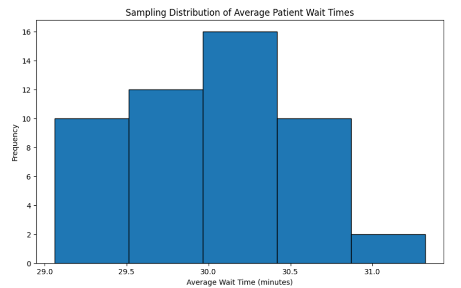
Suppose you want to understand the average spending of customers at a store. Instead of asking every single customer, you take several smaller samples and calculate the average spending for each sample. The collection of these sample averages forms what is known as the sampling distribution of the mean ( ).
).
The table below shows the collection of these sample means, which forms the sampling distribution of 
| Sample | Sample Size | Mean (x̄) |
|---|---|---|
| 1 | 100 |

|
| 2 | 100 |

|
| 3 | 100 |

|
| ... | ... | ... |
| 30 | 100 |

|
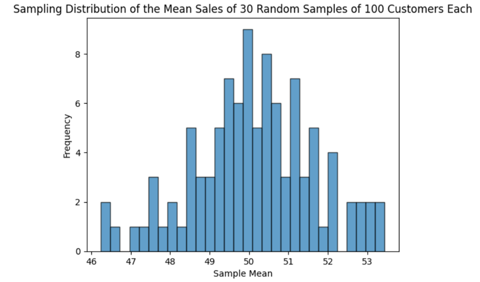
The histogram below is a plot of all the sample means from the table above. The histogram visualizes the distribution of the sample means. The histogram helps you understand the central tendency (average) and variability of the sample means.
The graphic below illustrates the construction of another sampling distribution of Even though the population mean is 82.5, the image visually demonstrates how the means of samples drawn from that population can vary. This sampling distribution of  consists of six samples, each with a sample size of 20.
")
Just as with other distributions we have studied, the sampling distribution of has its own mean, standard deviation, and shape.
Returning to the example of understanding the average spending of customers at a store, no information is available regarding the original population's spending patterns. However, this is acceptable due to the Central Limit Theorem, a statistical concept that offers insights into the sampling distribution of the sample mean ().
The Central Limit Theorem (CLT) provides you with information about the characteristics of the sampling distribution of The CLT tells us:
will be approximately normal (bell-shaped) if the sample size is large enough (at least 30 for most distributions). has its own mean and standard deviation. will have a mean equal to the population mean. is the population standard deviation divided by the square root of the sample size (this is called the standard error).

EXAMPLE
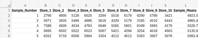
A retail chain wants to understand its average monthly sales across all its 250 stores to make informed business decisions. However, analyzing the average sales across all its stores is time-consuming and resource-intensive. Instead, the company asks you to use a sample-based approach to estimate the average monthly sales for all its 250 stores. shown in the spreadsheet below. The first five rows of the sampling distribution for sales_CLT.xlsx are shown below.
 , you can provide the company with an estimate of the average monthly sales across all 250 stores by using:
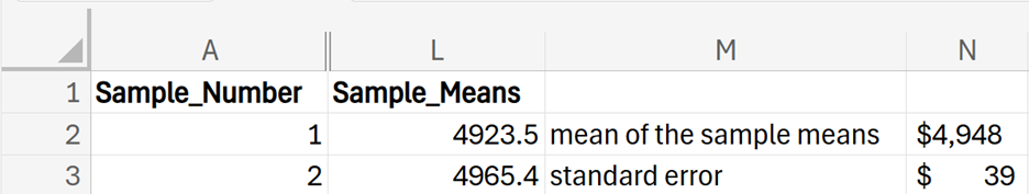
 can be found by taking the mean of the sample means in column L. In Excel, in cell N2, enter:
is $4,948. This gives the retail chain a reliable estimate of the average monthly sales across all stores. The mean of the sample means is a more reliable estimate of the population mean because it aggregates information from multiple samples, reducing the impact of any anomalies in individual samples. This is why the retail chain uses the mean of the sample to estimate the overall average monthly sales for all its stores.
can be found by taking the mean of the sample means in column L. In Excel, in cell N2, enter:
is $4,948. This gives the retail chain a reliable estimate of the average monthly sales across all stores. The mean of the sample means is a more reliable estimate of the population mean because it aggregates information from multiple samples, reducing the impact of any anomalies in individual samples. This is why the retail chain uses the mean of the sample to estimate the overall average monthly sales for all its stores.

 . That is, this value helps the retail chain understand how much the mean of the sample means ($4,948) is expected to vary from the true population mean. A smaller standard error indicates a more precise estimate of the population mean, μ.
 approaches a normal distribution as the sample size becomes large, regardless of the original population’s distribution. ) from the population, calculated as the standard deviation of the sampling distribution of that statistic.
The mean of the sampling distribution of is theoretically equal to the population mean, μ. However, in practice, there are several reasons why they might not be exactly the same. For instance:
will vary from sample to sample. This variability is natural and expected. The more samples you take, the closer the mean of the sampling distribution will get to the population mean, but with a limited number of samples, there will always be some difference. would converge to the population mean, μ. With a finite number of samples, there will always be some small difference. is not exactly equal to the population mean, due to some of the factors discussed above.

Imagine you’re working for a company that wants to know the proportion of employees who prefer working remotely versus in the office. Instead of asking every employee, you decide to survey a smaller group, or sample, of employees. The proportion of employees in your sample who prefer working remotely is called  . Now, if you took many different samples from your company, each sample would give you a different . The distribution of all these values from different samples is called the sampling distribution of the proportion (p̂).
The table below shows the collection of these sample proportions, which forms the sampling distribution of 
| Sample | Sample Size | Sample Proportion (p̂) |
|---|---|---|
| 1 | 100 |

|
| 2 | 100 |

|
| 3 | 100 |

|
| ... | ... | ... |
| 30 | 100 |

|
The histogram below is a plot of all the sample proportions from the table above. The histogram visualizes the distribution of the sample proportions. The histogram helps you understand the central tendency (average) and variability of the sample proportions.
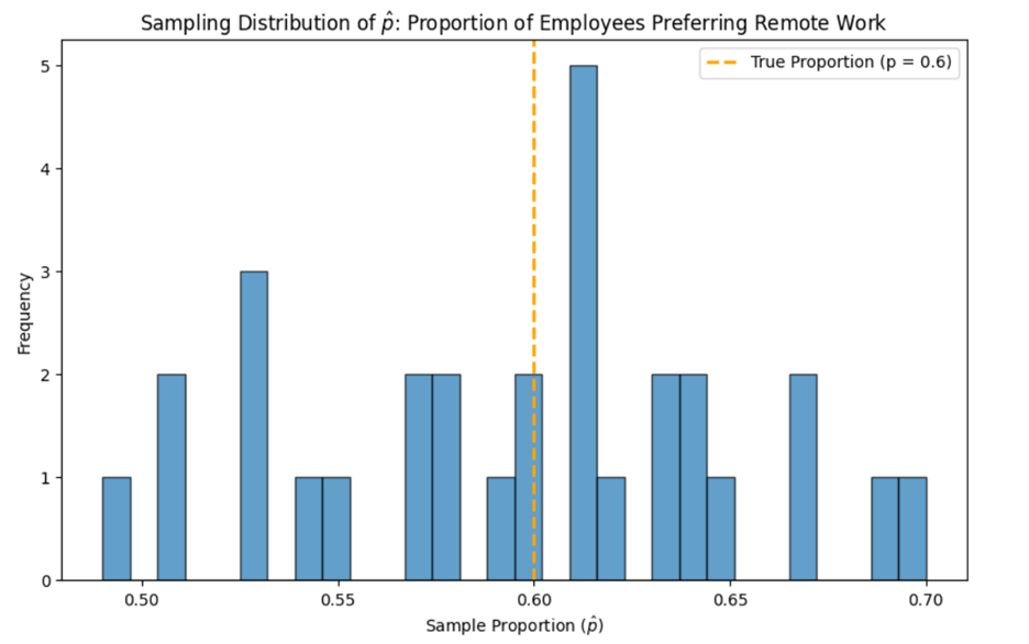
The histogram above was created with 30 samples of size 100. If you were to take 100,000 samples of size 100, the histogram would look like the following:
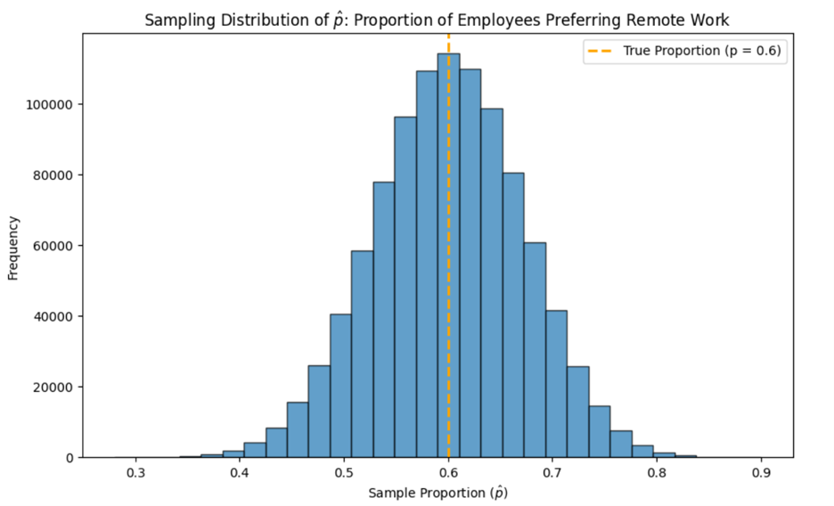
The reason the histogram becomes smoother and looks more like a normal distribution with more samples is due to the law of large numbers and the Central Limit Theorem working together. As you take more samples, the average of the sample proportions will converge to the population proportion. This means that with more samples, the overall distribution of sample means will better represent the true population mean.
The Central Limit Theorem states that the distribution of will approach a normal distribution as the sample size increases. However, this also implies that with a larger number of samples, the variability in the sample means decreases, making the distribution appear more normal.
Below are some key points about the sampling distribution of 
will approximate a normal distribution as the sample size becomes large. , a common rule of thumb is that the sample size, n, should be large enough such that both np and  are greater than 5, where p is the population proportion. This helps ensure that the normal approximation is valid. is equal to the true population proportion, p. This means that, on average, will be a good estimate of p. The formula for the mean of the sampling distribution of is:
  would be close to p. is called the standard error. It measures how much varies from sample to sample. The formula for the standard error of is:
  (the sample mean) and (the sample proportion) is that these distributions help assess how close the sample mean or proportion is to the true population mean or proportion. In other words, they indicate how accurate is as an estimate for μ (the population mean) and how accurate is as an estimate for p (the population proportion). These topics will be explored in more detail in future tutorials.
Source: THIS TUTORIAL WAS AUTHORED BY SOPHIA LEARNING. PLEASE SEE OUR TERMS OF USE.
A property that states the sampling distribution of  approaches a normal distribution as the sample size becomes large, regardless of the original population’s distribution.
A property that states as the size of a sample increases, the sample mean will become closer to the population mean and the sample proportion will become closer to the population proportion.
Distribution of a given statistic based on a random sample, showing how the statistic varies from sample to sample.
A distribution of all possible sample proportions of a given sample size from a population, showing how the sample proportion varies from sample to sample.
A distribution of all possible sample means of a given size from a population, showing how the sample mean varies from sample to sample.
Measure of the variability of a sample statistic (such as ) from the population, calculated as the standard deviation of the sampling distribution of that statistic.