Table of Contents |
If you recall from a previous lesson, normal distributions have density curves that are symmetric and bell-shaped. The mean, median, and mode of the normal distribution are all the same and equal to the center value of the density curve. However, there are situations where a distribution may not be symmetrical. We call these skewed distributions.
The first distribution that you see below is skewed to the right. It reflects a situation in which there would be many values concentrated toward the lower end of the distribution compared to the higher end. This is typically how the housing market is distributed.
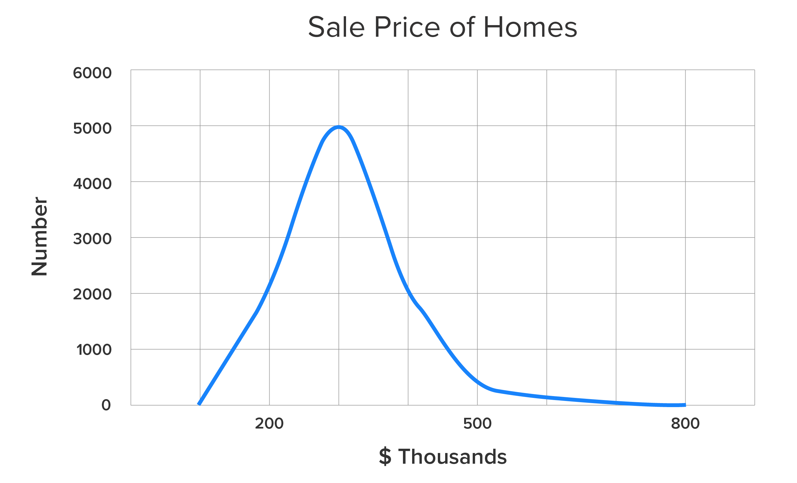
On the bottom (horizontal) axis, you have the price listed in thousands of dollars. The range is from around $100,000 up to almost $800,000. Most of the values are concentrated around $300,000. This is going to be a right-skewed, or positively skewed, distribution curve. A distribution having this shape is called a right-skewed, or positively skewed, distribution. It is defined this way because the peak is left of the center, but there is a wide range of prices that are much higher. These higher values will result in a mean and median that are both higher than the mode.
Consider the same distribution shown below.
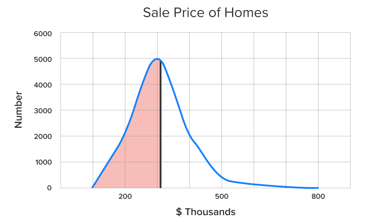
The vertical black line is drawn at the median of the distribution. We know this is the median since half of the distribution is to its left and the other half is to its right.
In addition, notice that the values are spread out more to the right of the median than they are to the left of the median. This suggests that the mean is higher than the median.
Another way to know that a distribution is right-skewed is that it has a “tail” in the right-hand direction. This “tail” represents the several higher home prices. Therefore, the direction of this tail also tells you the direction of the skew.
If you look at the distribution of the mileage of used cars shown below, you notice that there are similarities to the right-skewed graph from earlier, but this time, the peak is to the right of center, and the elongated tail is on the left side. This type of distribution is called a left-skewed distribution, or a negatively skewed distribution.
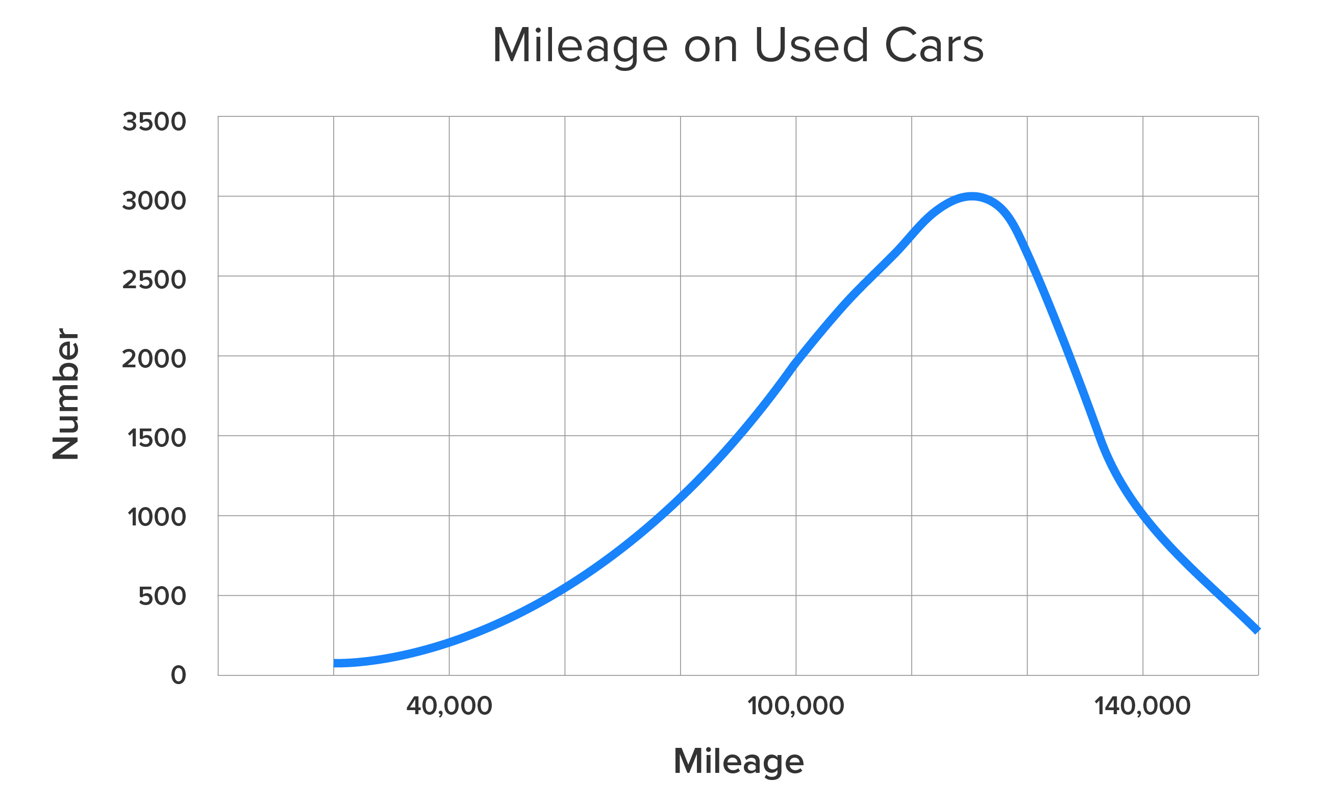
Notice that there are smaller frequencies of cars with lower mileage. This is due to people possibly waiting a lot longer to trade in their vehicles, which would suggest that they have higher mileage. This results in a left-skewed distribution. Notice that the tail points to the left, which emphasizes that the direction of the tail also tells us the direction of the skew.
Since a left-skewed distribution is essentially a mirror image of a right-skewed distribution, we would expect the relationship between the mean, median, and mode to be in reverse.
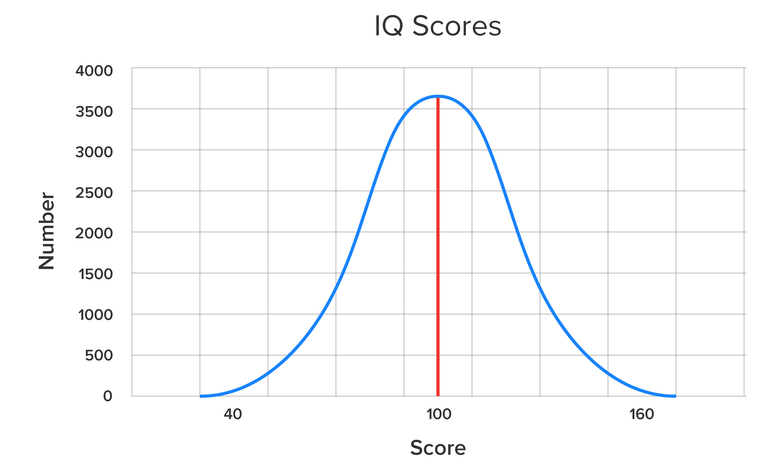
So, how do we identify differences between skewed distributions? Look at the graph above, which shows a normal distribution. It’s symmetrical, which means that the mean, median, and mode are identical, and correspond to the peak, which is in the center.
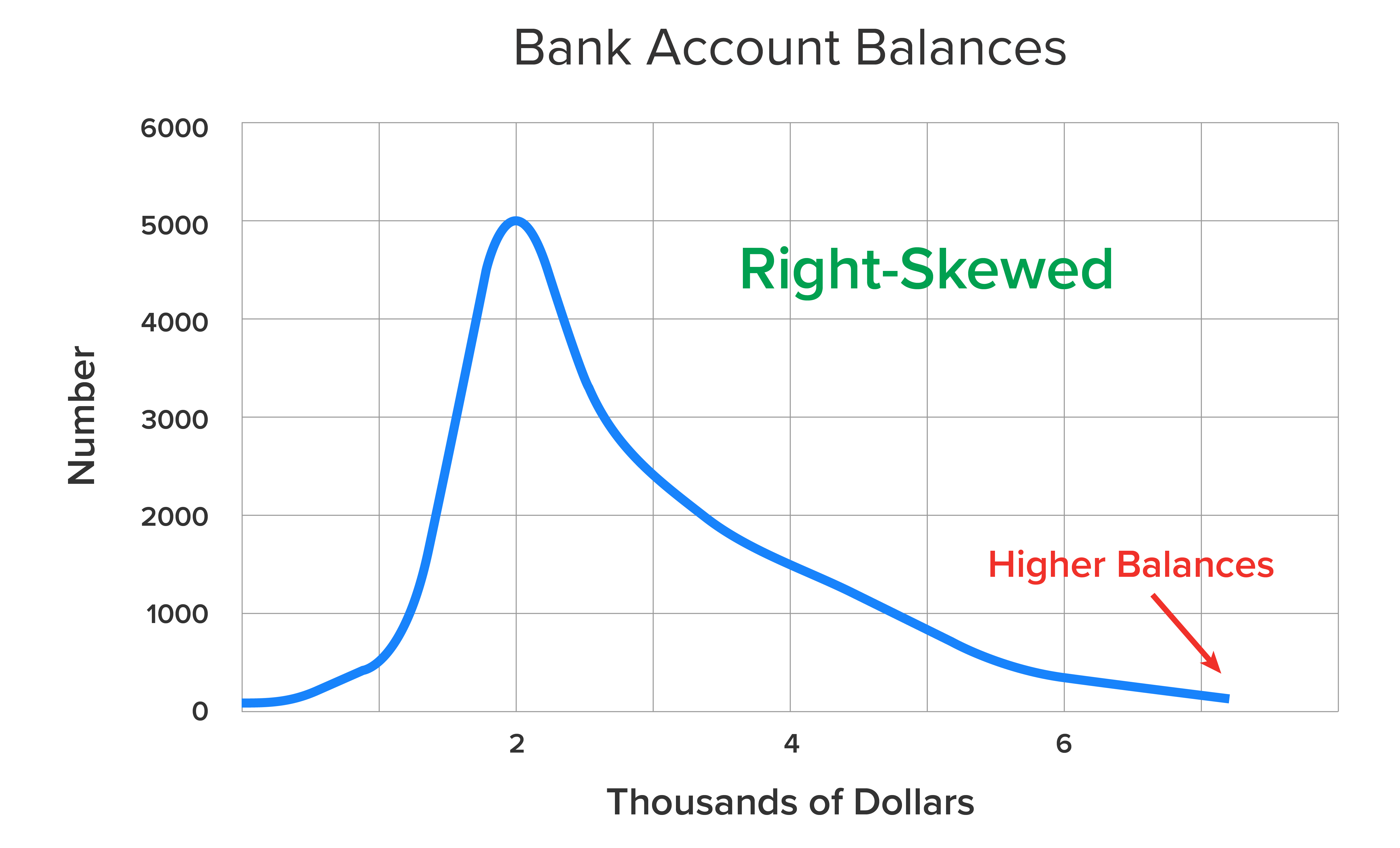
On one hand, bank account balances would likely have right-skewed distribution. Some people have quite a bit of money in their bank account, but many don’t. In this situation, the mode and the median are going to be relatively low, and the mean is going to be higher. That’s simply because there are some large balances that cause the mean to be larger than the mode and median.
On another hand, the useful life of a laptop would likely provide a left-skewed distribution. Consider the graph below:
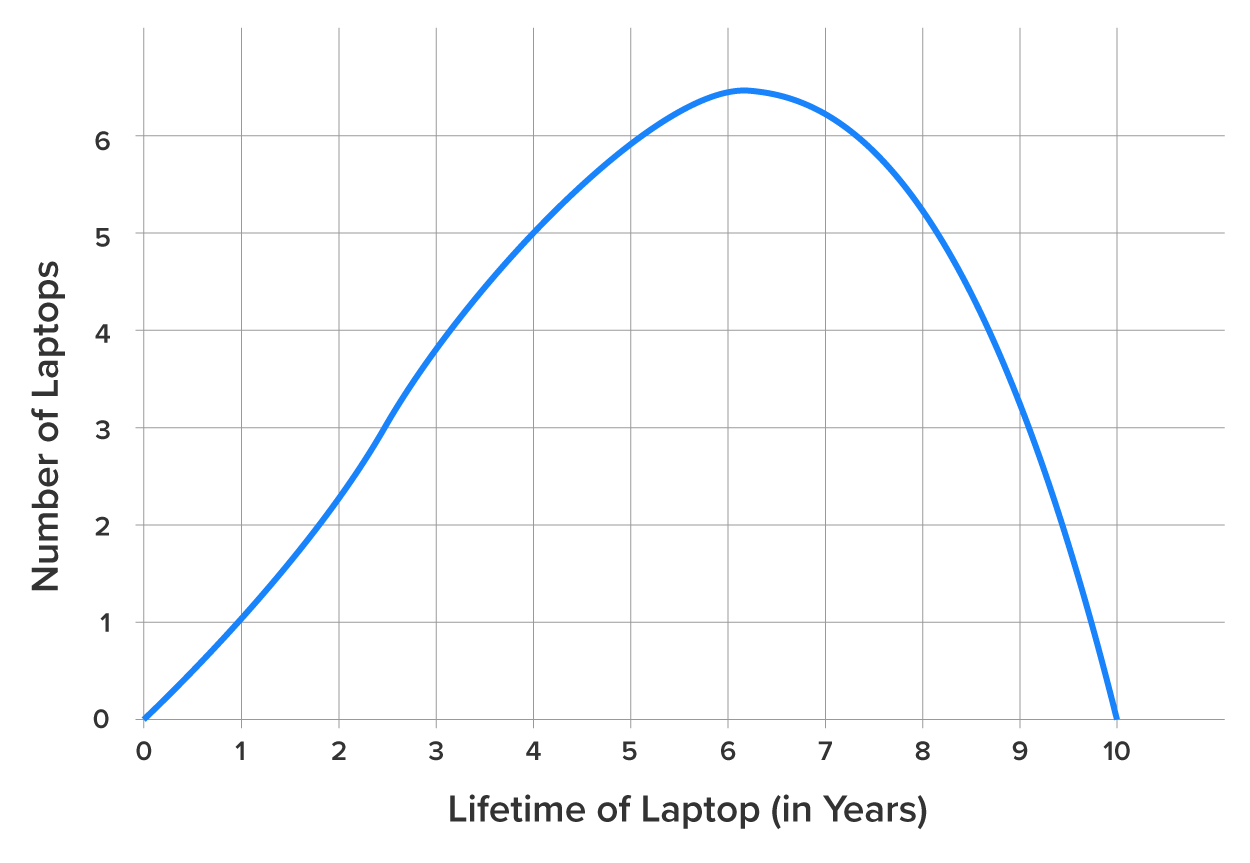
Based on this graph, most laptops last around 6 years, with some lasting longer (up to 10 years), and a tail to the left to represent the ones that didn’t last as long (down to less than a year). Naturally, you would not expect many to last less than a year, but the spread of values to the left of the mode (6 years or so) is far more than the spread to the right.
| Situation | Skewness |
|---|---|
| Mean < Median < Mode | Left |
| Mean = Median = Mode | Normal (Bell-Shaped) |
| Mode < Median < Mean | Right |
Source: This work is adapted from Sophia author Dan Laub.