Regression Analysis

before you start

This tutorial provides a gentle introduction to simple linear regression. In an upcoming unit, there will be more details and examples related to regression. For now, concentrate on how simple linear regression is applied in business, including grasping what simple linear regression entails, its business applications, and how analyzing different components of the model aids in the interpretation of the results in the context of the business problem.

1. Simple Linear Regression

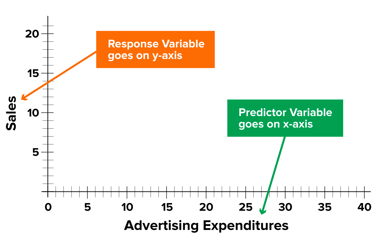
Simple linear regression is a statistical model that allows you to summarize and study the relationship between two variables. The term ‘simple’ in simple linear regression means there are only two variables involved. The variables are:

• x: the predictor, explanatory, or independent variable. This tutorial refers to x as a predictor. x may be a quantitative or categorical variable.
• y: the response, outcome, or dependent variable. This tutorial will refer to y as the response.

Simple linear regression is named from the fact that the model is a linear one, meaning it assumes the relationship between x and y is linear.

Not all relationships will be linear. However, the regression ideas in this tutorial can be applied to whatever function best describes the data (exponential, logarithmic, etc.)

term to know

Simple Linear Regression

A statistical model used to estimate or predict the relationship between two variables.

1a. The Straight Line and Simple Linear Regression

The equation of a straight line is generally written as:

• y is the response variable
• x is the explanatory variable
• m is the slope
• b is the y-intercept

• y is the response variable
• x is the explanatory variable
• is the slope
• is the y-intercept

did you know

Greek letters are used to denote population parameters, and lowercase letters represent sample statistics.

1b. Fit the Simple Linear Regression Model to the Data

The first step in constructing a simple linear regression model is to fit the data to the model. This is done using a mathematical procedure called ordinary least squares (OLS).

Working for a retail company, you may want to predict future sales based on how much is spent on advertising. Using collected historical data on sales and advertising expenses, the ordinary least squares (OLS) method is used to fit a simple linear regression model. By understanding and applying OLS, this analysis can provide valuable insights into how advertising spend impacts sales, helping the company allocate its marketing budget more effectively.

OLS finds estimates of the intercept and slope for the model so that it accurately represents the observed data as shown in the figure below. OLS determines the slope and y-intercept of the regression line, which minimizes the difference between predicted and actual values. The difference between the predicted and the actual values is known as residuals Each residual is the distance between a data point and the point predicted for that x value by the linear regression model (ŷ). OLS will find the linear line that is as close to the data points as possible.

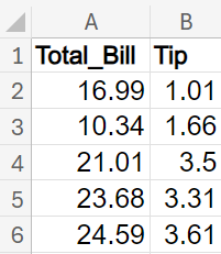
Suppose you want to predict the tip amount from a lunch bill from a restaurant. You have collected the total lunch bills and the amount of the tip from a local restaurant in your city. The table below shows the data.

try it

1. Open the tips.xlsx file.



In this scenario, the response (y) is tip and the predictor variable (x) is total_bill.

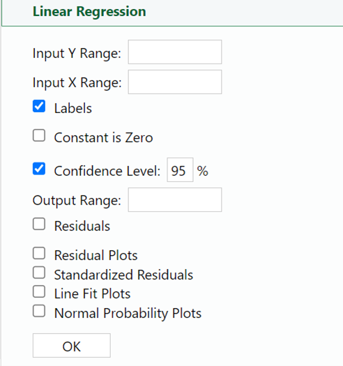
2. To build the simple linear regression model in Excel, select Linear Regression in the XL Miner Analysis Toolpak. The Linear Regression dialog box opens.



3. Put your cursor in the Input Y Range box. Then use your mouse to select the tips data that are in rows B1 to B6 (including the tip column label value in row B1). Once you have selected all the data, the Input Y Range value should now show rows B1 to B6 selected.

Input Y Range: $B$1:$B$6

4. Repeat this same process for the Input X Range box and select the data for the total_bill column. Once you have selected all the data, the Input X Range should not show rows A1 to A6 selected.

Input X Range: $A$1:$A$6

5. The Output Range box specifies where you want the regression output to be displayed. Let’s output the regression results in the same worksheet as our data. Click into the Output Range box and select any cell in the worksheet.

6. Select the Residuals checkbox so the residuals will be in the regression results. Select OK.

7. You will see that you obtain three components of the output: SUMMARY OUTPUT, ANOVA, and RESIDUAL OUTPUT. Let’s parse through what we need to evaluate the regression model.

First, the estimated parameters of the model can be found under the ANOVA output in the Coefficients column as shown below.

The table below shows the estimated values of the intercept and the slope

Coefficients
Intercept ()	-0.526450834
Total_bill ()	0.162739408

8. Using these values, you can now specify the model as:

9. You can use the model to predict the amount of tip for a particular bill value. For example, if you wanted to know what the predicted amount of the tip would be for a $20 bill, perform the following:

Great work! Now you have a formula for a line that best represents your tip and bill data. In the next section, we will return to this example to assess the model fit. Specifically, we will be returning to the section of your output called ANOVA.

watch

Follow along with this video to predict the tip amount from a lunch bill from a restaurant using linear regression. The predicted value of the tip that you observe in step 9 above and in the video will be different in the decimal places due to the rounding of the hand computation shown in step 9 above.

terms to know

Ordinary Least Squares (OLS)

A mathematical procedure that estimates the parameters in a linear model.

Residual

The difference between the predicted value of the response and the actual value of the response variable. Also a synonym for error.

2. Sum of Squares

A business may want to predict the tip amount based on the total bill. The linear regression analysis could help in understanding the relationship between the two variables more quantitatively, which could be useful for restaurant management to predict future tips and plan accordingly. However, the sum of squares determines the model fit, which helps to assess how well the regression line represents the data by quantifying the variability the model does and does not account for.

To determine how well this line fits the data, you calculate three values known as the sum of squares:

Let’s look in more detail at each of these parts:

• Sum of Squares Total (SST): In more general terms, SST measures the total amount of variability in the y variable (the response) around the mean (ȳ).

hint

Remember, the Σ sign means summation, that is to “add up” or “sum together” a series of numbers. The SST formula above is using Σ to indicate the sum of the squared differences between each observed response value () and the mean of the observed response values (ȳ). The index variable is i. would be the first value of the response variable in the data, would be the second value of the response variable in the data, and would be the last value (the nth value) of the response variable in the data.

When you compare data points to the mean (average) of the response value, you’re using the mean as a basic model to predict the response. If you didn’t have any other model, the mean would be a decent guess because it represents the average outcome.

Steps:

• Using the Mean as a Model: Think of the mean as a simple way to predict the response. For example, if you want to predict tips, you could just use the average tip amount.
• Calculating SST: The Total Sum of Squares (SST) measures how much the actual data points differ from this mean. It does this by:
  • Finding the difference between each data point and the mean.
  • Squaring these differences (to avoid negative values canceling out positive ones).
  • Adding up all these squared differences.

• Large SST: If SST is large, it means the data points are far from the mean, indicating that the mean is not a good predictor.
• Small SST: If SST is small, it means the data points are close to the mean, indicating that the mean is a good predictor.

• Sums of Squares Regression (SSR): SSR represents the deviation of predicted values from the mean of the response variable.

• What It Does: SSR measures how well the model’s predictions compare to the mean (average) of the response variable. For example, SSR measures how well the model’s predictions (predicted tips) compare to the mean (average tip).
• Large SSR: If SSR is large, it means the model’s predictions are far from the mean and closer to the actual data points. This indicates the model is doing a good job of predicting the response variable.
• Small SSR: If SSR is small, it means the model’s predictions are close to the mean and not much better than just using the mean itself. This indicates the model is not doing a good job of predicting the response variable.

• Good Model: A large SSR means the model explains a lot of the variability in the data, making it a good predictor.
• Poor Model: A small SSR means the model doesn’t explain much of the variability, so you might as well just use the mean to predict the response.

• Sums of Squares Error (Residuals) SSE: This measures how much the predicted values (tips) differ from the actual observed values (tips). It represents the error in the model’s predictions.

The relationship between the three sums of squares is The total amount of variability in the response variable around the mean is the variability that the model accounts for (SSR) and the amount of variability the model does not account for (SSE). So, SST shows the overall variability, SSR shows how much of that variability your model explains, and SSE shows how much your model misses.

The coefficient of determination, often denoted as , is a measure that tells you how well your regression model explains the variability of the response variable. Here’s a simple explanation:

Coefficient of Determination ():

• What It Is: is a number between 0 and 1 that indicates how well your model’s predictions match the actual data.
• How It’s Calculated: is calculated using the sums of squares we discussed earlier:

Keep in mind that these are general rules, and you need to keep the context of the analysis in mind when determining a threshold for what constitutes a good model fit to the data.

Now let’s look at how you could apply the sum of squares to help you assess a simple linear regression model in Excel.

try it

Continuing with the tips.xlsx file from the previous example or using tips2.xlsx which contains the linear regression model, assess the model fit using the sum of squares.

Using the calculations from above, we specified the model as:

The sum of squares values are in the ANOVA output as well. The table below shows the sum of squares values. The column labeled SS is the sum of squares.

ANOVA
	df	SS	MS	F	Significance F
Regression	1	3.594103	3.594103	5.014615	0.111030188
Residual	2	2.150177	0.716726
Total	3	5.74428

The SST value is 5.74, SSR is 3.59, and SSE is 2.15. Notice that SSR and SSE add up to SST.

To interpret the sum of square values, it will be helpful to calculate the average of y (tip amount). The mean of y can be found with the AVERAGE() function in Excel.

=AVERAGE(B2:B6)
=2.618 or 2.62

The SST value of $5.74 quantifies the amount of variability there is in the tip amounts without considering any predictors. $5.74 is how much the tips deviate from the average tip amount of $2.62.

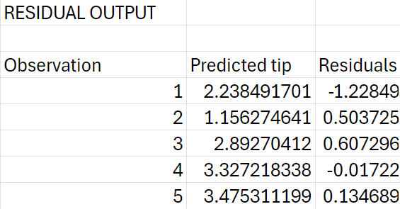
For both SSR and SSE, you must have the predicted values of the tips In the regression output under the RESIDUAL OUTPUT, the predicted values are provided. For each data point, you obtain the predicted value (Predicted tip column) and the residuals (Residuals column).



You can verify the first predicted value by substituting the corresponding x value into the model for each observation.

For the first data point, the bill_amount (x) value is $16.99. So, to obtain the predicted value of the tip for this observation, substitute the $16.99 value for x in the model.

In Excel, the predicted value of the tip is $2.24. The hand computations are different due to rounding the Excel results to 2 decimal places. The predicted tip for the first lunch bill is $2.19 (rounded).

The SSR value of $3.58 quantifies the amount of variability that the regression model accounts for when you compare the predicted values to the mean amount of tips.

And lastly, SSE provides you the sum of the squared residuals. In the RESIDUAL OUTPUT, the column named Residuals contains the residual for each data point. You can verify the first residual by confirming:

The difference between the first residual you observe in Excel (-1.23) and the hand-computed residual is a rounding error from using two decimal places. The first residual value of $-1.18 means that the model underestimated the tip amount by $1.18.

SSE is the sum of the squared residuals, and its value is $2.15 from the ANOVA portion of the Excel output. $2.15 represents the amount of variability in the tip amounts that the regression model cannot quantify.

To determine what proportion of improvement beyond using the mean the regression model provides, you can calculate

63% of the variability in the amount of tips can be accounted for (explained) by the simple linear regression model. The value is in the SUMMARY OUTPUT portion of the Excel output.

watch

Follow along with this video to assess the model fit using the Sum of Squares for our linear regression model predicting the tip amount from a lunch bill from a restaurant.

did you know

The coefficient of determination, is the square of the correlation coefficient, That is,

terms to know

Sums of Squares

An umbrella term to denote the three key sum of squares measures used to evaluate how well the regression model fits the data.

Sums of Squares Total (SST)

The total variability of the response variable around the mean.

Sums of Squares Regression (SSR)

Quantifies the variability explained by the regression model.

Sums of Squares Error (Residual) (SSE)

Quantifies the unexplained variability between the predicted values and the actual value of the response variable.

Coefficient of Determination

Measures the proportion of variability in the response variable that can be explained using the predictor variable.