Table of Contents |
Finally, we have arrived at the point where we can draw some conclusions about profitability! You’ve learned about production, which input combinations minimize cost, and how to analyze costs. You’ve also examined revenue to confirm that sales revenue has been maximized. If the firm has minimized its cost and is maximizing its sales revenue, then the chances are good that it is maximizing its profit. But rather than guess, let’s review a couple of techniques to confirm that profit has been maximized.
Going forward economic profit will be referred to as total profit (TP), which is total revenue (TR) minus total cost (TC), where both implicit and explicit cost and revenue are assumed to be included.

Let’s return to our strawberry business. C&C Family Farm’s owners are eager to know if their business is profitable. The data in the table reports total profit (column 4), which is the difference between total production costs (column 3) and total sales revenue (column 2).
In the first row, note that total profit is a negative value (-$100). It is possible for a business venture to incur losses in the short run. Can you determine the source of the loss from the table?
|
Total Output (Q) (in Pounds) (1) |
Total Revenue (TR = P * Q) (2) |
Total Cost (TC = FC + FV) (3) |
Total Profit (TP = TR - TC) (4) |
|---|---|---|---|
| 0 | $0.00 | $100.00 | -$100.00 |
| 100 | $167.00 | $200.00 | -$33.00 |
| 230 | $384.10 | $300.00 | $84.10 |
| 290 | $484.30 | $400.00 | $84.30 |
| 350 | $584.50 | $500.00 | $84.50 |
| 380 | $634.60 | $600.00 | $34.60 |
| 400 | $668.00 | $700.00 | -$32.00 |
Notice in row one the total output (column 1) is zero. No strawberries were picked. If C&C Family Farm did not produce any output, then it had nothing to sell. However, the total cost is the sum of both fixed cost (FC) and variable cost (VC). If no strawberries were picked, then C&C Family Farm also hired no workers, which is the variable input and the source of variable cost. If we subtract variable cost from total cost at zero output, then it leaves fixed cost. The source of the negative total value is the cost of C&C Family Farm’s lease on its 20-acres and the interest being paid on the purchase of the tractor and wagon. Recall that fixed cost is incurred whether a business produces output or not. Fixed cost doesn’t go away until the end of the contract.
In row two the business is also experiencing a loss (-$33), but a much smaller loss than in row one (-$100). It is a smaller value because C&C Family Farm earned some revenue ($167) to help offset the cost of $200. After row two, the loss becomes profit, before becoming negative again at 400 pounds of strawberries produced. Did you notice that total profit is not increasing at every level of output? It seems to have peaked at an output level of 350 pounds of strawberries.
Let’s plot both total revenue and total costs against the total output to help visualize C&C Family Farm’s profit situation. In the graph below, the two totals cross between 100 and 200 pounds of strawberries. Before this crossing point, total cost is greater than total revenue. Remember that we are still carrying the fixed cost. But the fixed cost is now being spread over larger and larger quantities of output, so its value is becoming smaller and smaller as output increases. Beyond this output level, total revenue is greater than total costs, at least until it reaches about 400 pounds of production where production costs–specifically, the variable cost paid for variable inputs–rises sharply. As the firm increases output more variable inputs are purchased.
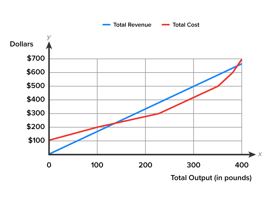
Are you able to calculate the total profit from the graph? Suppose we examine the vertical distance between the two lines at each level of production. At zero pounds of total output, the vertical distance between total cost and total revenues is -$100, the fixed cost. At 300 pounds the distance is a little less than $100. If you review the table, you can confirm your dollar value estimates. Since profit is total revenue minus total cost, wherever total revenue and total cost are the greatest vertical distance apart along an output line, this is where total profit will be the largest.
Finding the difference between total revenue and the total cost is one way of determining if a firm is profit-maximizing: just look for the largest positive value in the total profit column of the table. The problem, though, is that this method is not precise enough to tell us how to change the level of output to improve profit. Should the firm increase or decrease production–and by how much–to reach the profit-maximizing level of output? Fortunately, there is an alternative to considering the difference between the totals: using the profit maximizing rule, which you will learn about in the following section.
In economics, marginal analysis is key to understanding how to maximize profit. Most analyses about decision-making in economics follow a simple rule: equate the margins. People naturally compare costs and benefits and think total costs and total benefits are the deciding factor in making decisions. In truth, in order to make an optimal decision, you must compare how costs and benefits change from one unit to the next. Examining the added benefit and added cost of choosing a little more or a little less of something is known as marginal analysis. Think of marginal analysis as the analysis of change from one unit to the next.
Let’s consider C&C Family Farm’s margins. The table below reports marginal revenue and marginal cost for the strawberry business. Beginning in row two, where output is 100 pounds of strawberries (column 1), marginal revenue (column 2) represents the change in total revenue divided by a change in total output. Except for row one, marginal revenue is the same for all levels of output. Plotting this data will result in a horizontal marginal revenue curve.
|
Total Output (Q) (In Pounds) (1) |
Marginal Revenue (MR = Change in TR / Change in Total Output) (2) |
Marginal Cost (MC = Change in TC / Change in Total Output) (3) |
|---|---|---|
| 0 | - | - |
| 100 | $1.67 | $1.00 |
| 230 | $1.67 | $0.77 |
| 290 | $1.67 | $1.67 |
| 350 | $1.67 | $1.67 |
| 380 | $1.67 | $3.33 |
| 400 | $1.67 | $5.00 |
Except for row one, marginal cost (column 3) is reported. The marginal cost is $1.00 for 100 pounds of strawberry production, then it drops to $0.77 in row two. From there on, marginal cost rises. The rise in marginal cost after 230 pounds of production is expected, because we are increasing the number of workers, our variable input, and the source of rising cost in the short run.
As you review the information in the table above, think about the shape of the marginal cost curve that can be plotted from this data. Review the graph below in which the values for marginal revenue and marginal cost are plotted against total output. When marginal revenue is the same for all levels of output, we get a horizontal MR curve (blue). The somewhat J-shaped MC curve (red) has the expected shape. How can this information help the firm determine how to maximize profits?
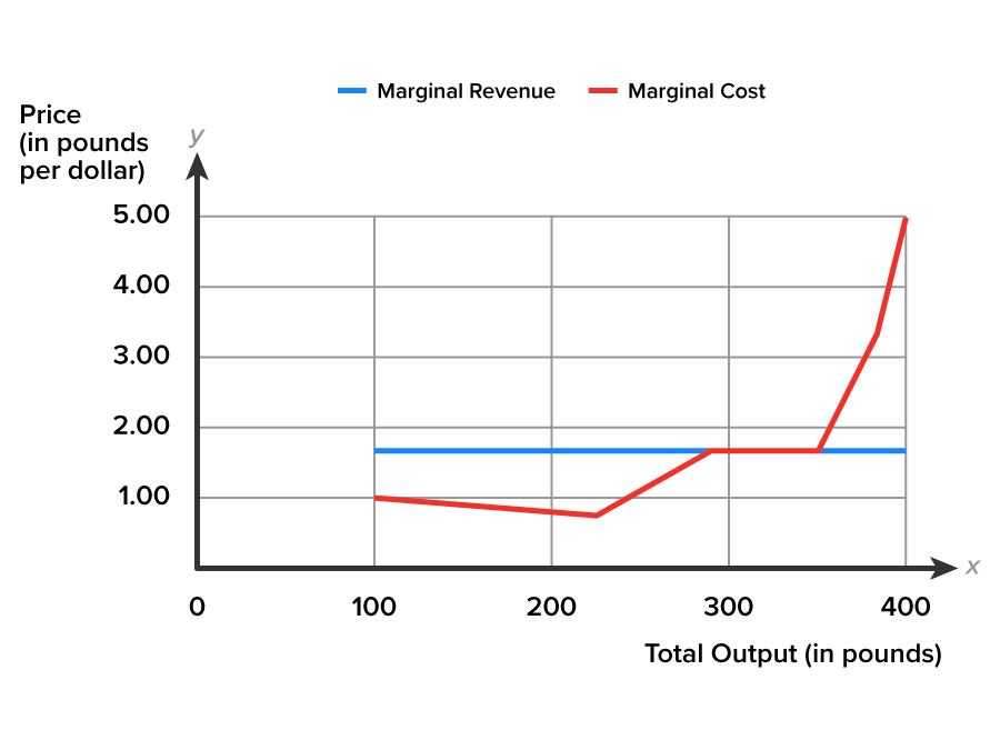
If the firm follows what is known as the profit-maximizing rule of equating the margins, then it will produce at the level of output that maximizes profit. It cannot do better!
At all output levels before MR = MC, you can see that MR > MC. What this means is the firm can do better by increasing its production level to maximize its profits. Producing one more unit is going to add more to revenue than to cost–and increase profit.
EXAMPLE
Suppose you are selling six T-shirts and marginal revenue is $20, while marginal cost for the sixth shirt is $12. This means that the sixth T-shirt added $8 to profit, because $8 more went to revenue than to cost. Therefore, you want to continue producing as long as marginal revenue is greater than marginal cost.Any output level beyond MR = MC means MC > MR. What this means is the firm can do better by reducing its production level to maximize profits. Producing one less unit is going to reduce the cost and increase profit.
EXAMPLE
When you produce the ninth T-shirt, the marginal revenue is $20, while the marginal cost of the ninth shirt is $25. This means that the ninth T-shirt reduced profit by $5. Five more dollars went to cost than to revenue, so profit would fall by $5. Therefore, you would want to scale back production to MR = MC.Since MR = MC between the levels of production of 290 and 350 pounds of strawberries, does it matter whether C&C Family Farm chooses to operate at 290 pounds of production or 350? Let’s think this through. Does it cost any more to produce 350 pounds versus 290?
Remember, we are looking at the margin, the per unit additional cost of producing one more unit of output. There is no difference in the per unit marginal cost of producing 291 versus 349 pounds. What about marginal revenue? Again, the per unit additional revenue for producing 291 pounds or 349 pounds is the same per unit. The optimal decision, then, is to produce at the higher of the two production levels.
C&C Family Farm has all the information needed to select the profit-maximizing level of output of approximately 350 pounds of strawberries, and to charge a price of $1.67.
By choosing 350 pounds as its production level in the short run, the combination of production inputs has been decided. The firm will be minimizing total costs. At 350 pounds of output, the firm will maximize its sales revenue given the price of $1.67 per pound. C&C Family Farm is doing the best it possibly can to maximize profits.
A word of caution. This analysis is built upon the assumption that everything else remains unchanged for C&C Family Farm. What could possibly change? The going price in the strawberry market could fall or rise. The temperature could drop and freeze the strawberry plants. The market for strawberries could dip if consumer preferences change unfavorably. Other possibilities include a change in any of the other non-price factors we learned about in the lesson about demand and supply.
Source: THIS TUTORIAL WAS AUTHORED BY SOPHIA LEARNING. PLEASE SEE OUR TERMS OF USE.
