Production: Marginal

1. Marginal Product of Labor

Now that you’ve learned about total and average products, let’s explore how an additional worker affects output. The marginal product of labor (MPL) represents the additional output obtained from the addition of one worker to the production process. Mathematically, marginal product is calculated as the change in total product divided by the change in labor. You performed similar calculations in the lesson about marginal utility.

formula to know

Marginal Product of Labor (MPL)

In the table below, notice that the total product of labor for the first worker is 100 pounds of strawberries. This is because with zero workers, there is no total product at all, so hiring the first worker increases the total product from zero. To calculate the marginal product of labor, determine the change in total output (column 3) by subtracting the quantity of pounds in row two from the quantity of pounds in row one (100-0). Then determine the change in number of workers (column 2), by subtracting the number of workers in row two from the number workers in row one (1-0). Then divide the change in total product (100-0) by the change in labor (1-0). As you can see, worker one has a marginal product of labor of 100 pounds, and worker two has a marginal product of labor of 120 pounds. Use the MPL formula to complete the calculations for rows four through eight of the table below. Another version of this table with the formulas completed for all the rows appears further along in this lesson.

We can repeat the process to determine the marginal product of each of the subsequent workers. To calculate the marginal product of labor for the second worker:

• Subtract the total product in row three from the quantity of pounds in row two (220-100).
• Then subtract the number of workers in row three from the number workers in row two (2-1).
• Divide the change in total product (220-100) by the change in labor (2-1).

try it

Suppose in your business the 40 workers produce 2400 units of output, while 100 workers produce 3000 units.

What is the marginal productivity of labor?

Notice that hiring the second worker produces an additional 120 pounds of strawberries. That’s good news! The first worker had to work alone, and to perform all the tasks involved in picking strawberries without assistance. Hiring a second worker allows for sharing some of the work. Perhaps the second worker is stronger than the first, which made carrying the strawberry cartons off the field less difficult. So while the second worker carries the cartons, the first worker concentrates on picking the berries off the vine. When workers focus on particular tasks for which they are particularly well-suited within the overall production process, it is called specialization. The marginal product of labor increases when workers specialize, because workers are doing tasks for which they are better suited or trained.

EXAMPLE

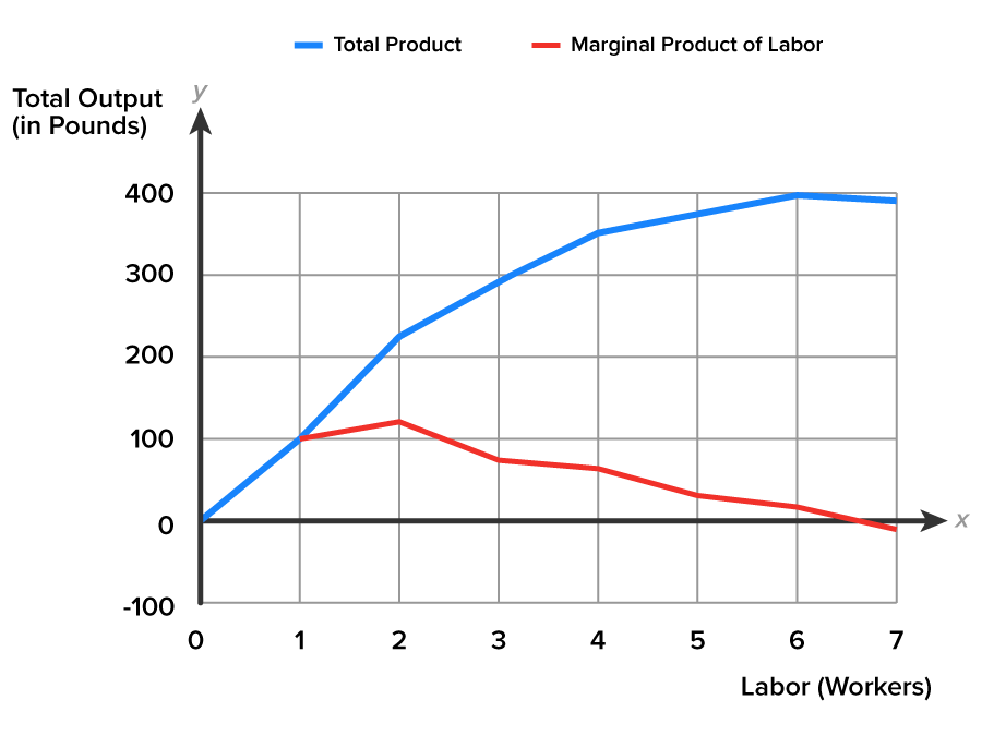
Suppose you live with two other people. Each week you agree that three tasks must be completed: the dishes need to be washed, the yard needs to be mowed, and the laundry must be done. Because you love the outdoors, you agree to care for the yard. The other two individuals then each choose a task that they feel best fits them. Each person specializes by focusing on the tasks for which they are well-suited. By doing this, all tasks are accomplished, and each task is completed with the least expenditure of resources: time, energy, and effort.

term to know

Marginal Product of Labor (MPL)

The additional output obtained from the addition of one more worker.

Specialization

When workers focus on the particular tasks for which they are well-suited within the overall production process.

2. Marginal Product Curve

We can visualize the relationship between the number of workers and output by plotting the data from the table. The number of workers is on the horizontal axis (x-axis), and the total output is on the vertical axis (y-axis). The total product curve (blue) shows the relationship between the quantities of total output that can be obtained from the different number of workers. The relationship between the change in the quantities of total product between two rows, and the change in the number of workers for the same two rows, is represented as a marginal product curve.

The marginal product curve (red) lies below the total product curve (blue). It begins with the first worker. The marginal product curve peaks on the second worker and then it falls. The marginal product curve passes through the horizontal axis at zero, and turns negative between the sixth and seventh workers.

What’s going on here? We know that allowing workers to specialize in the task for which they are best suited will boost output. But continuing to add workers beyond a certain number–in this case beyond two workers–causes the marginal product of labor to decline until it eventually turns negative. Why? Because in the daily production operation the only resource being allowed to change is the number of workers–not the acreage of land. The strawberry farm has leased 20 acres. It’s fixed in size. Adding more and more workers to the 20 acres reduces the amount of space any one worker has available to work. At some point, perhaps, the workers spend more time in idle chatter than actually picking strawberries. That certainly does not produce output!

EXAMPLE

A two-person saw works much better with two timber cutters than with one. Suppose we add a third timber cutter. What will that person’s marginal product be? What will that person contribute to the team? Perhaps the third worker can oil the saw's teeth to keep it sawing smoothly, or bring water to the two people sawing. While it is helpful to keep the workers hydrated and the saw oiled, it does not produce any cut logs.

Let’s review the marginal product column in the table again. The marginal product curve peaks at worker two. Notice that after the second worker, the marginal product of labor is positive but declining. But hiring the seventh worker actually results in a negative marginal product (-10), representing a decrease in the marginal productivity.

term to know

Marginal Product Curve

The relationship between the change in the quantities of total output and the change in the number of workers.

3. The Law of Diminishing Marginal Productivity

What we have seen demonstrated in both the table and in the graph is an important observation about production in the daily operation of a business: adding workers to a production process increases the marginal product of labor at first, but sooner or later additional workers will have a decreasing, though still positive, effect on the marginal product of labor. After a certain point, added workers contribute smaller and smaller increases to total output. Eventually, hiring additional workers may have no effect, or even a negative effect, on total output.

This phenomenon is a common pattern in economics. The law of diminishing marginal productivity states that increasing one input, while keeping everything else the same, will initially increase overall production–but beyond a certain point, further additions of that variable input will produce smaller and smaller increases. Diminishing marginal productivity is very similar to the concept of diminishing marginal utility that we learned about in the lesson on consumer choice and utility. Both concepts are examples of the more general principle of diminishing marginal returns.

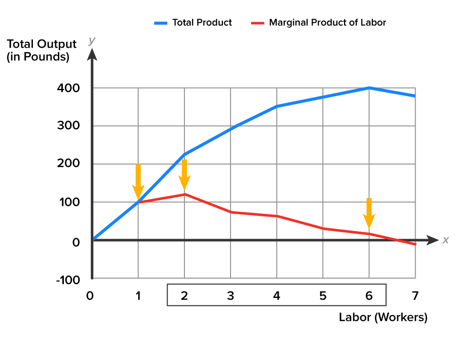
Productivity is positive, but decreasing, in the region of the graph between workers two and six in the table where diminishing marginal productivity sets in. Why? As in the case of strawberry pickers, adding more workers (a variable input when all other inputs are fixed) creates a crowding out problem. Crowding out occurs when workers have less and less access to other inputs. Consider crowding out in the context of C&C Family Farm. We have examined the effect of adding up to seven workers to the 20-acre field. What is likely to happen to the ratio between workers and acreage as even more workers are hired? With 10 workers there is approximately two acres of work space per worker. With 20 workers the work space per worker drops to one acre. The ratio becomes more unfavorable, reducing the ability of an additional worker to make a positive contribution to output.

reflect

Have you ever worked in a business where you spent time chatting with your coworkers? How do you think that this affects office productivity—your productivity and the productivity of your coworkers? Imagine that you work in a 15 by 15 office without cubicles and with two rows of desks and work spaces that are three feet apart. What would be the ideal number of workers for the space? What would be likely to happen throughout the day as workers become restless, and move about the workspace? Would workers get more or less work done as colleagues chat with one another? One would expect productivity of workers to fall. Production is replaced with non-productive activity. This is another explanation for declining productivity.

We have accounted for specialization boosting the MPL, when workers perform tasks they are best suited for. We have accounted for the diminishing marginal productivity effect caused by continuing to add a variable input, workers, to a fixed input, the 20 acres of land. We have not explained why an added worker might cause MPL to turn negative, as in the case of adding worker seven to the production process. This third region of the MPL curve occurring between workers six and seven indicates a seriously adverse relationship between the fixed (20 acres of land) and the variable inputs (number of workers). The added output has become negative. What would you imagine happening if 5000 workers were added to the 20 acres of strawberries?

Let’s summarize what we have learned. In the graph below, notice that the red marginal product curve below has three distinct regions of interest.

1. The first region at the intersection of the marginal product line intersects with the total product line, and occurs between one and two workers where increasing marginal productivity occurs due to specialization. The far left arrow notes where this region begins. This region extends to worker two.
2. The second region occurs between workers two and six where marginal product peaks and then begins to diminish, due to the effect of crowding out. The center arrow indicates where this region begins. This region extends to worker six.
3. The third region occurs where the total product has peaked, and the marginal product of labor passes through the horizontal zero axis and turns negative. The arrow on the right indicates where this region begins. It extends to worker seven.

Diminishing marginal productivity occurs when a production process relies on both fixed and variable inputs. There are only 20 acres of strawberry fields. There is only one two-person saw. Will it always be this way? Not necessarily. C&C Family Farm might purchase or lease more acres in the future, at which point hiring a seventh worker may add positively to total output. Or the timber cutters might buy a new saw and hire a fourth worker to increase output. But that is not the decision for today.

terms to know

Law of Diminishing Marginal Productivity

An economic principle that shows that increasing one input while keeping everything else the same will initially increase overall production but beyond a certain point further additions of that input will produce smaller and smaller increases.

Crowding Out

A problem caused by adding more of a variable input when other inputs are fixed.

4. Putting It Together: How Many Workers to Hire?

Let’s examine the productivity data for C&C Family Farm, and decide the optimal number of workers to hire for harvesting the 20-acre plot of strawberries.

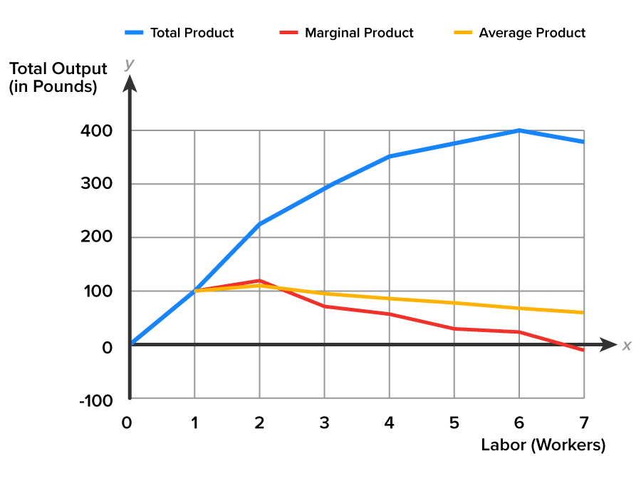
If we were to focus only on the total product, then, maybe, hiring six workers would be optimal. After all, total output increases to 400 pounds, until the total product curve peaks at worker six. If we focus on the average product, then we might want only two workers, whose average productivity is 110 pounds. The average product curve peaks at worker two, and is positive but diminishing for all workers after worker two.

As you can see in the graph below, between one and two workers, the marginal product of labor is rising faster than the average product of labor. The marginal product of labor curve is above the average product of labor curve in the graph. The next worker adds more output than the average product of each worker.

Focus on the marginal product curve. Notice that it peaks at worker two where the added output of the second worker is 130 pounds. At this point the marginal product of labor is positive, but as the line continues the marginal product of labor diminishes, until it turns negative.

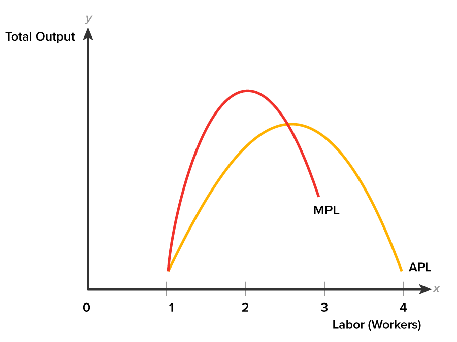
To help you better see the relationship between MPL and APL, consider the graph below. The MPL curve intersects the APL curve at its maximum point (two workers and 110 pounds of output). Thereafter, both MPL and APL fall.

So we return to the original question: what is the optimal number of workers to hire given C&C Family Farm’s 20-acre plot of strawberries? Unfortunately, we can't answer that question just yet! We can’t determine the optimal number of workers to hire, because we need information about the cost of the inputs–we need to know how much we are paying each worker, and we need to know the cost of the 20-acre field, as well as the cost of any equipment being used.

Production and cost have an inverse relationship. The cost of producing output depends on the amount of inputs required, and the price of each input. Today, the firm decides which factors of production to purchase and in what combination so as to minimize its production costs. In the first lesson of the next Challenge, we will distinguish between the types of inputs, before examining costs.