Optimization Models

1. Introduction to Optimization Models

Optimization models are tools that help us find the best solution to a problem while considering certain limits or rules. These models are very important in business data analytics because they help companies make smart decisions that save money, improve efficiency, and boost overall performance.

In the world of business data analytics, optimization models are part of prescriptive analytics. While descriptive analytics looks at what happened in the past, diagnostic analytics explains why it happened, and predictive analytics tries to guess what will happen in the future, prescriptive analytics suggests actions to achieve the best results. Optimization models are a key part of prescriptive analytics because they provide clear recommendations on how to solve complex business problems.

term to know

Optimization Models

Mathematical models used to determine the most effective way to achieve a specific goal, given a set of constraints or conditions.

1a. Importance of Optimization Models

Optimization models are crucial in business data analytics because they help companies make smart decisions. By using these models, businesses can:

• Save Money: Find the most cost-effective ways to operate.
• Improve Efficiency: Streamline processes to get better results with less effort.
• Boost Performance: Achieve goals more effectively and stay competitive.

2. Key Components of Optimization Models

Understanding the key components of optimization models is essential for effectively using them to solve business problems. These components include the objective function, decision variables, and constraints. Each of these elements plays a crucial role in defining and solving optimization problems.

2a. Objective Function

The objective function is a mathematical expression that defines the goal of an optimization model. It tells us what we want to achieve, such as minimizing costs or maximizing profits. For example, if a company wants to minimize transportation costs, the objective function will represent the total cost of transportation.

To create an objective function, you need to:

1. Identify the goal (e.g., minimize costs, maximize profits).
2. Determine the factors that affect this goal (e.g., transportation costs, production costs).
3. Write a mathematical expression that combines these factors to represent the goal.

Minimize:

term to know

Objective Function

The mathematical function that will either be minimized or maximized in an optimization model.

2b. Decision Variables

Decision variables are the values that you can control in an optimization model. They represent the choices needed to be made to achieve the objective. For example, in a transportation problem, decision variables could be the number of units to ship from each warehouse to each store.

To identify decision variables, ask yourself:

1. What choices do you need to make to achieve the goal?
2. What values can you control in the model?

term to know

Decision Variables

The controllable factors in an optimization model that influence the outcome of the objective function.

2c. Constraints

Constraints are the limits or rules that the solution must follow. There are different types of constraints, such as:

• Equality Constraints: These require that two expressions are equal. For example, the total number of units shipped from a warehouse must equal the number of units available.
• Inequality Constraints: These require that one expression is greater than or less than another. For example, the number of units shipped to a store cannot exceed its demand.

1. Identify the limits or rules that must be followed.
2. Write mathematical expressions that represent these limits.

terms to know

Constraints

Conditions or limits that must be satisfied in an optimization model.

Equality Constraints

Conditions that require two expressions to have the same value.

Inequality Constraints

Conditions that require one expression to be greater than or less than another.

3. Types of Optimization Models

Throughout this course, you will explore three types of optimization models: linear programming, integer linear programming, and nonlinear programming. A description and short introduction to each of these optimization models is provided in the upcoming sections.

3a. Linear Programming

Linear programming (LP) is an optimization model used to find the best solution to a problem where the relationships between variables are linear. A linear relationship means that the change in the outcome is directly proportional to the change in the input. For example, if you double the number of products produced, the total cost will also double. Linear programming involves maximizing or minimizing a linear objective function, subject to a set of linear constraints.

To illustrate a linear objective function, consider the following example.

EXAMPLE

Consider a company that produces two products: A and B. The company wants to maximize its profit. The profit from each unit of Product A is $10, and the profit from each unit of Product B is $15. The objective function to maximize profit would be:

Maximize:

In this linear objective function, the decision variables (A) and (B) are not squared or raised to any exponent. The relationship between the number of products produced and the total profit is a straight line. If you double the number of products, the profit also doubles. This straightforward, proportional relationship is a key characteristic of linear functions.

The graph below shows the linear relationship between the number of products produced (A and B) and the total profit, illustrating how profit increases proportionally with the production of each product.



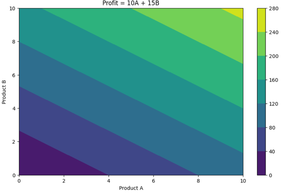
In this graph:

• The x-axis represents the number of Product A produced.
• The y-axis represents the number of Product B produced.
• The colors represent the total profit, with lighter colors indicating higher profits.

This visual helps illustrate how the profit increases proportionally with the number of products produced, maintaining a linear relationship. For example, if you look at the graph, you can see that producing 5 units of Product A and 5 units of Product B results in a certain profit level of:

Doubling the production to 10 units of Product A and 10 units of Product B doubles the profit:

which is a clear indication of linearity.

Note: In this example, you assume that the number of units of Product A and Product B are equal. This assumption is made for simplicity and to clearly illustrate the linear relationship. However, in a real-world scenario, the quantities of Product A and Product B may vary independently, and additional constraints may be applied to the model.

term to know

Linear Programming (LP)

An optimization model in which the objective function and constraints are linear.

3b. Integer Linear Programming

Integer linear programming (ILP) is a special type of linear programming where some or all the decision variables are required to be integers. This is particularly useful in situations where the variables represent discrete items, such as people, machines, or products, which cannot be divided into fractions.

In ILP, the objective function is a linear equation that you aim to either maximize or minimize, like linear programming. However, what sets ILP apart is that the constraints, which are also linear equations or inequalities, include conditions that require some or all of the decision variables to be integers.

Let’s consider an example of integer linear programming.

EXAMPLE

Suppose a retail company is planning a promotional campaign and needs to decide how many email and social media ads to run. Each email ad reaches 1,000 customers, and each social media ad reaches 500 customers. The company wants to reach exactly 5,000 customers, and they can only run whole ads (no fractions).

In this scenario, the decision variables are the number of email and social media ads to run. The company wants to find the combination of ads that will reach all the customers without exceeding the required number.

For example, the company might consider running 3 email ads and 2 social media ads. This would reach:

• 3 email ads × 1,000 customers/email ad = 3,000 customers
• 2 social media ads × 500 customers/social media ad = 1,000 customers
• Total = 3,000 + 1,000 = 4,000 customers

Since 4,000 customers are less than 5,000, this combination does not work. The company needs to find another combination that exactly meets the requirement of 5,000 customers.

After trying different combinations, they might find that running 4 email ads and 2 social media ads works perfectly:

• 4 email ads × 1,000 customers/email ad = 4,000 customers
• 2 social media ads × 500 customers/social media ad = 1,000 customers
• Total = 4,000 + 1,000 = 5,000 customers

This combination meets the requirement, ensuring that the company reaches exactly 5,000 customers.

term to know

Integer Linear Programming (ILP)

A type of optimization model where the objective function and constraints are linear, but the decision variables are restricted to integer values.

3c. Nonlinear Programming

As you have seen in a previous example, linear programming involves maximizing or minimizing a linear objective function, where the relationship between the decision variables is straightforward and proportional. Now, let's explore nonlinear programming (NLP), which deals with optimization problems where the objective function or any of the constraints are nonlinear.

In NLP, the relationships between variables can be more complex, involving quadratic, cubic, exponential, or logarithmic terms. This complexity allows for a broader range of real-world applications but also makes the problems more challenging to solve.

Let’s look at a nonlinear objective function using the following example.

EXAMPLE

Consider a company that wants to maximize customer satisfaction based on the number of products A and B produced. Customer satisfaction increases with the number of products, but at a decreasing rate due to market saturation. The objective function might look like this:

Maximize:

In this nonlinear objective function, the 10A and 15B terms represent the initial positive impact of producing products A and B on customer satisfaction. However, the and terms introduce the concept of diminishing returns, where satisfaction increases at a slower rate as production grows. These negative squared terms model real-world effects like market saturation and resource constraints, reducing the objective value as production continues to increase.

Nonlinear functions can take many forms, such as involving squared terms, higher-order polynomials, or exponential and logarithmic relationships. In this particular case, the nonlinearity arises because the decision variables (A and B) are squared, which creates a curved solution space rather than a flat one seen in linear functions.

This means the relationship between the number of products produced and customer satisfaction is not a straight line. Initially, increasing production significantly boosts customer satisfaction. However, as more products are produced, the additional satisfaction gained diminishes—reflecting a classic case of diminishing returns. This occurs due to factors such as market saturation or consumer fatigue.

The presence of squared terms or other higher-order exponents makes the function nonlinear and more complex. The graph below shows the nonlinear relationship between the number of products produced (A and B) and customer satisfaction, illustrating how satisfaction increases with production, but at a decreasing rate.

Market saturation occurs when supply meets or exceeds customer demand, meaning that producing additional units yields diminishing returns in customer satisfaction. In this example, as more products are produced, the incremental satisfaction from each new unit decreases because the market can only absorb so much. Once most customer needs are met, producing more products has little impact on overall satisfaction.

In the graph, the curved lines reflect the nonlinear nature of the relationship, where satisfaction initially rises quickly but then slows as production increases—highlighting the diminishing returns effect.



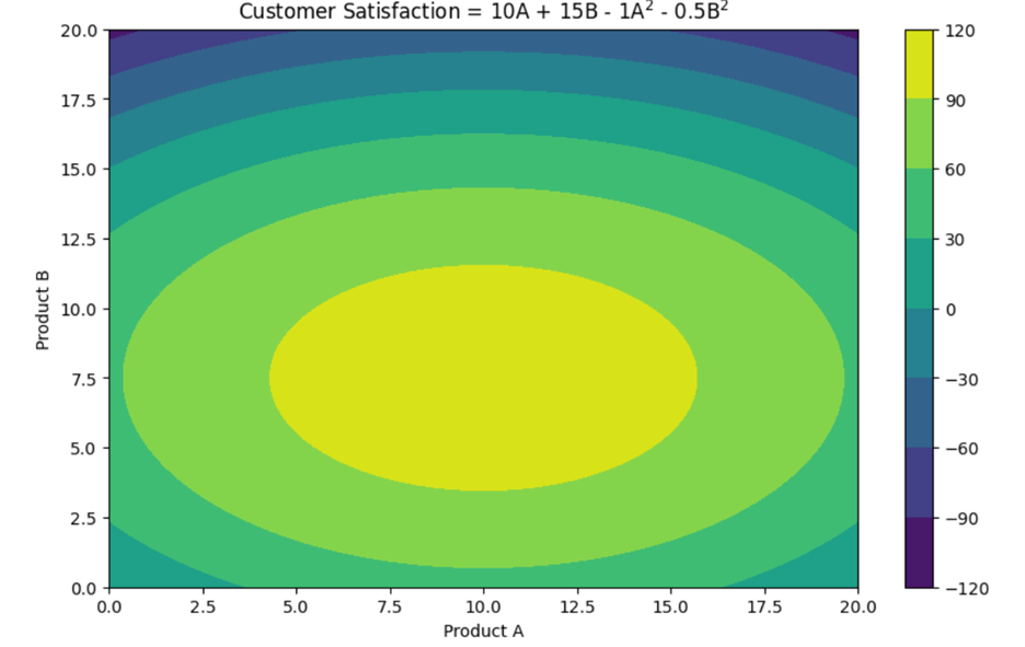
In this graph:

• The x-axis represents the number of product A produced.
• The y-axis represents the number of product B produced.
• The colors represent customer satisfaction, with lighter colors indicating higher satisfaction levels.

This visual illustrates how customer satisfaction increases as more products are produced, but at a decreasing rate, reflecting the nonlinear relationship. For example:

Producing 5 units of product A and 5 units of product B results in:

Doubling production to 10 units of both product A and product B does not double satisfaction:

These calculations show that while satisfaction increases, the rate of increase slows as production grows—clearly demonstrating the effect of the squared terms and the nonlinear nature of the relationship.

terms to know

Nonlinear Programming (NLP)

A type of optimization model where the objective function or constraints involve nonlinear relationships, such as exponential terms.

Diminishing Returns

The principle that as more resources or input are added, the resulting gains or benefits increase at a decreasing rate.

3d. Comparison of the Three Types of Optimization Models

The table below highlights the key differences and similarities between the three types of optimization models that you have been introduced to in this tutorial. Each has its own unique features and applications, making them suitable for different types of problems.