One-Sample Hypothesis Testing - Means

before you start

This lesson builds on key concepts from an Introduction to Statistics course. Specifically, this tutorial assumes familiarity with the foundational idea of one-sample hypothesis tests for population means.

1. Introduction to One-Sample Hypothesis Testing for a Mean

In various business data analytics applications, determining whether a single group’s mean differs from a known value is often necessary. For instance, a company might want to check if its average salary differs from the industry average. This can be assessed using a one-sample hypothesis test for the mean.

A one-sample hypothesis test for the mean is a statistical method used to compare the mean of a single sample to a known population mean. This test helps determine if the observed sample mean is significantly different from the hypothesized population mean, or if the difference could be due to random variation.

Recall in the last tutorial, steps were provided to perform a hypothesis test.

1. State the Hypotheses: Clearly define the null and alternative hypotheses.
2. Gather the Data: Gather data in a way that is designed to test the hypotheses.
3. Choose the Significance Level: Decide on the α level (for example, 0.05 or 0.10).
4. Perform a Statistical Test: Use an appropriate statistical test to analyze the data. Common tests include t-tests, z-tests, and ANOVA.
5. Make a Decision: Based on the test results, decide whether to reject or fail to reject the null hypothesis. This decision is guided by a p-value, which indicates the probability of observing the data if the null hypothesis is true.
6. Interpret the Results: Explain the results of the hypothesis test in the context of the business problem.

There are three types of hypothesis tests for a mean. Each one is discussed in the upcoming sections.

1a. Two-Tailed Hypothesis Test for a Mean

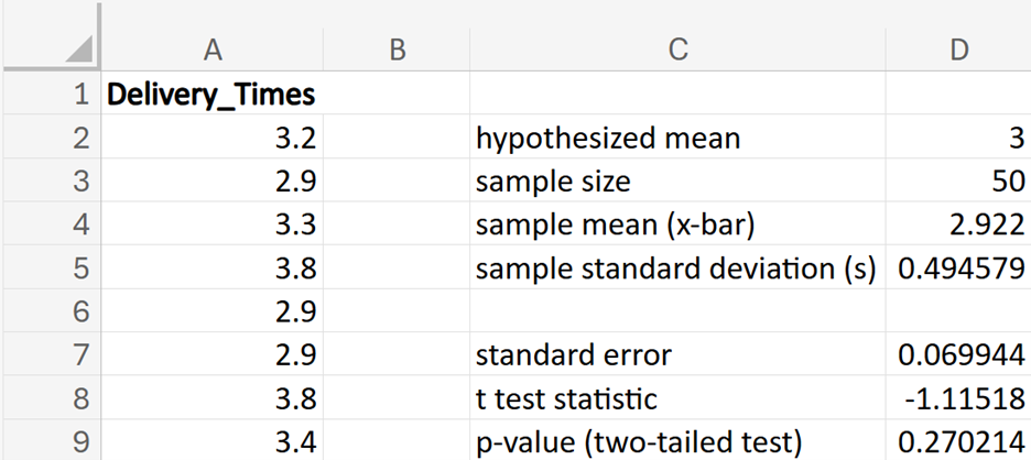
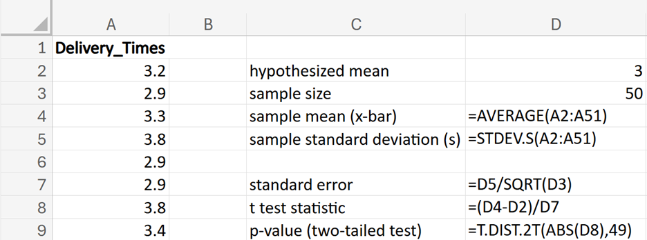
Let us walk through a practical example of performing a two-tailed hypothesis test for a mean.

EXAMPLE

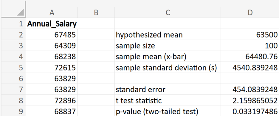
Tech Innovators Inc. is a rapidly growing technology company known for its innovative products and dynamic work environment. The company prides itself on offering competitive salaries to attract top talent. Recently, the HR department has raised concerns that the average annual salary of employees might have deviated from the industry average of $63,000. To address this concern, the company has decided to conduct a hypothesis test to determine if there has been a significant change in the average annual salary of its employees.

As a business data analyst, you have been tasked with performing a hypothesis test using the salary data of Tech Innovators Inc. to determine if the average annual salary has changed from the industry average of $63,000.

In performing this hypothesis test, you will complete the following steps.

Step 1: State the Hypotheses

• H₀:
• H₁:

Step 2: Gather the Data

In Excel, you have a sample of 100 Tech Innovators employee salaries. Using the data in Excel, you find:

• (sample mean; average value of the employee salaries in the sample)
• (sample standard deviation; amount of variability in the sample of employee salaries)
• (sample size; number of observations in the sample)

Step 3: Choose a Significance Level

Use a level of significance,

Step 4: Perform a Statistical Test

Since the population standard deviation, σ, is not known, you will use a t-test for this hypothesis test.

The t-test requires a test statistic to be computed. The test statistic is given by where μ₀ is the hypothesized mean in the null hypothesis, $63,500 in this example. This test statistic tells you how many standard deviations the sample mean is from the hypothesized mean of $63,500.

A test statistic of 2.16 means that the sample mean is 2.16 standard deviations above the hypothesized population mean. This large value suggests that the difference between the sample mean and the hypothesized population mean, μ₀, is quite substantial. In other words, the sample mean is far enough from the hypothesized mean that it suggests there may be a meaningful difference between the two.

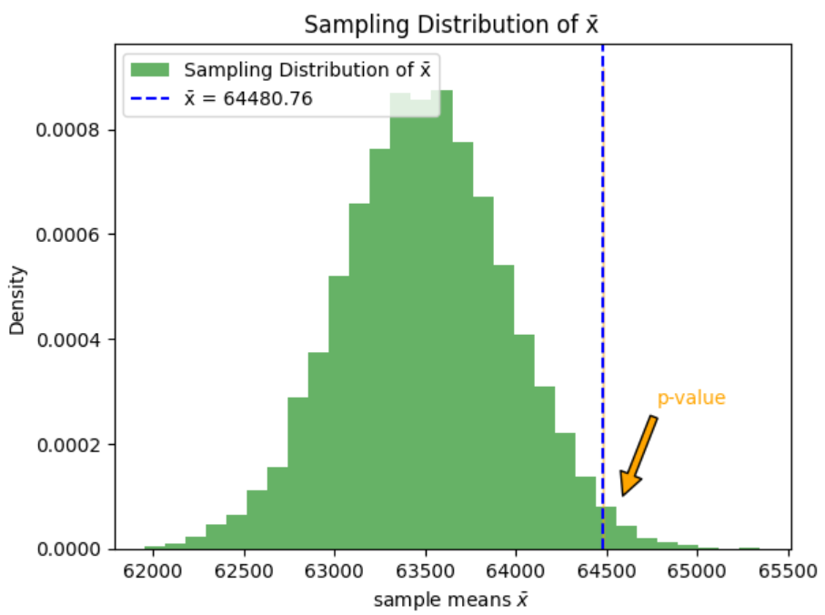
The test statistic directly relates back to the sampling distribution of The green histogram below represents the distribution of sample means if you repeatedly sampled from the population with a mean of The sampling distribution of is centered around the hypothesized mean of and has a standard deviation (standard error) of

The blue dashed line at $64,480.76 represents the sample mean, The area to the right of the blue dashed line represents the p-value, which is the probability of obtaining a test statistic as extreme as, or more extreme than, the observed test statistic (2.16) if the null hypothesis were true.



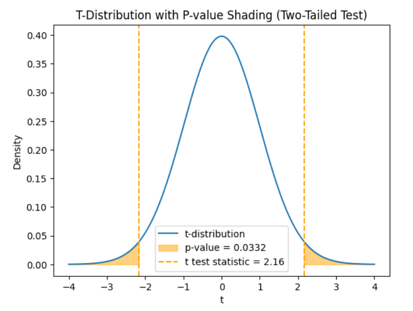
The t-distribution is used to standardize the sample mean, to account for the sample size and variability. The test statistic (t) is a point on the t-distribution, indicating how many standard deviations is from the hypothesized mean, You use the t-distribution to find the p-value for the hypothesis test. The graph below shows the t-distribution for a two-tailed hypothesis test. The orange dashed lines at and show the observed test statistics. The orange shaded areas represent the p-value, indicating the probability of observing test statistics as extreme as or more extreme, under the null hypothesis.



In a two-tailed test, you look for extreme values on both ends of the distribution, because you want to see if the sample mean is significantly different from the hypothesized mean (either higher or lower).

So, you have two critical values:

• One at for the high end.
• One at for the low end.

You will now use Excel to find the p-value for this two-tailed hypothesis test. Using the data in the employees_salaries.xlsx file, perform the following.

1. In cell C2, enter hypothesized mean. In cell D2, enter 63500.

2. In cell C3, enter sample size. In cell D3, enter 100.

3. In cell C4, enter sample mean (x-bar). In cell D4, enter the following formula:

=AVERAGE(A2:A101)

4. In cell C5, enter sample standard deviation (s). In cell D5, enter the following formula:

=STDEV.S(A2:A101)

5. In cell C7, enter standard error. In cell D7, enter the following formula:

=D5/SQRT(D3)

6. In cell C8, enter t test statistic. In cell D8, enter the following formula:

=(D4-D2)/D7

7. In cell C9, enter p-value (two-tailed test). In cell D9, enter the following formula:

=T.DIST.2T(D8,99)

In cell D9, you should obtain a p-value of 0.0332.

The T.DIST.2T() Excel function is used to calculate the two-tailed p-value of the t-distribution. The first argument is the value of the test statistic and the second argument is the degrees of freedom for the t-distribution, which is

Your Excel spreadsheet should contain these values for all of the computations.



Using Excel, you find the p-value to be 0.0332.

Step 5: Make a Decision

Since the p-value (level of significance), you can reject the null hypothesis.

Step 6: Interpret the Results

Since the p-value (0.0332) is less than the significance level (0.05), you reject the null hypothesis. This means there is sufficient evidence to conclude that the mean salary of Tech Innovators employees is significantly different from $63,500.

For guidance, the Excel formulas are shown in the screenshot below.

try it

An e-commerce company wants to ensure that the average delivery time for their orders is consistent with their target delivery time of 3 days. They collect a random sample of delivery times (in days) for recent orders to test if the average delivery time has deviated from the target.

The random sample is in the Excel file named e-commerce_delivery_times.xlsx. The delivery times are measured in days using a decimal form. The decimal part of the number of days is the number of hours on that particular day. For example, 3.2 means 3 days and 2 hours.

Using the data in the e-commerce_delivery_times.xlsx Excel file, perform a hypothesis test to determine if the average delivery time for all orders at the e-commerce company is significantly different from the target delivery time of 3 days. Use a level of significance of 0.05. Interpret the results of the hypothesis test.

Solution:

Null and alternative hypotheses:

• H₀:
• H₁:

Using Excel, you find the p-value for this test to be 0.2702. The Excel worksheets with the values of the test statistic and p-value are provided below.



You notice that the test statistic is a negative value for this problem, -1.12, meaning that the sample mean of 2.92 days is 1.12 standard deviations below the hypothesized mean of 3 days.

If the test statistic is negative, you will need to enclose the t test statistic in the ABS() function (absolute value) in Excel when using the T.DIST.2T() function to find the p-value.

The Excel worksheet with values and formulas is shown below:



Interpretation: Since the p-value (0.2702) is greater than the significance level (0.05), you fail to reject the null hypothesis. Based on the sample of delivery times collected, you do not have enough statistical evidence to conclude that the average delivery time for all packages is different from 3 days.

watch

Follow along with this video on analyzing average delivery time with a two-tailed hypothesis test.

term to know

Test Statistic

A standardized value calculated from sample data for a hypothesis test that measures how much your sample data deviates from the null hypothesis.

1b. Excel T.DIST() Functions for Calculating P-Values for Hypothesis Tests for Means

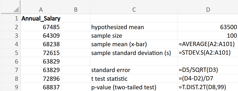
This table provides a guide on which Excel T.DIST() function to use for calculating p-values in different types of t-tests. It includes functions for two-tailed, right-tailed, and left-tailed tests, specifying the appropriate function and a brief description of each. The value of t in the table represents the test statistic.

1c. Right-Tailed Hypothesis Test for a Mean

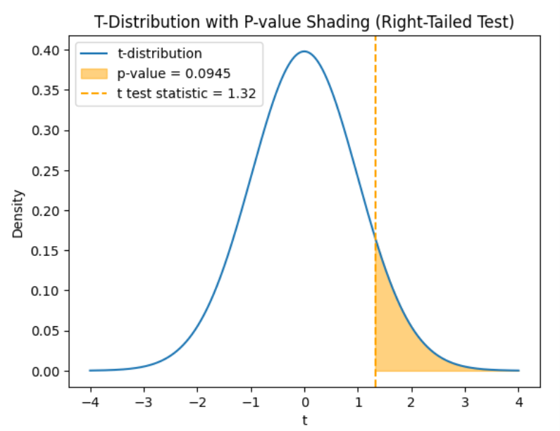
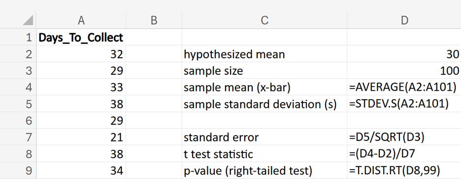
Let’s walk through a practical example of a right-tailed hypothesis test for a mean.

EXAMPLE

Financial Solutions Inc. is a well-established financial services company that prides itself on efficient operations and strong financial health. One key performance metric the company monitors closely is the average number of days it takes to collect accounts receivable. Historically, the company has maintained an average collection period of 30 days. Recently, there have been concerns that this period might have increased, potentially impacting cash flow and operational efficiency.

As a business data analyst, you have been tasked with analyzing the accounts receivable collection data to determine if the average number of days to collect accounts receivable has increased from the historical average of 30 days.

In performing this hypothesis test, you will complete the following steps.

Step 1: State the Hypotheses

• H₀:
• H₁:

Step 2: Gather the Data

In Excel, you have a sample of the number of days it took to collect accounts receivable for 100 different accounts. Using the data in Excel, you find:

• 
• 
• 

Step 3: Choose a Significance Level

Use a level of significance,

Step 4: Perform a Statistical Test

Once again, since σ is not known, you will use the t-test to conduct this test. The test statistic is given by where μ₀ is the hypothesized mean in the null hypothesis, 30 days in this example.

A test statistic of 1.32 means that the sample mean is 1.32 standard deviations above the hypothesized population mean.

You use the t-distribution to find the p-value for the right-tailed hypothesis test. The graph below shows the t-distribution for a right-tailed hypothesis test. The orange dashed line at shows the observed test statistic. The orange shaded area represents the p-value, indicating the probability of observing the test statistic, or something more extreme, if the null hypothesis is true.



In a right-tailed test, you look for extreme values to the right end of the distribution, because you want to see if the sample mean is significantly greater than the hypothesized mean.

You will now use Excel to find the p-value for this right-tailed hypothesis test. Using the data in the accounts_receivable_collection_days.xlsx file, perform the following.

For guidance, the Excel formulas are shown in the screenshot below.



1. In cell C2, enter hypothesized mean. In cell D2, enter 30.

2. In cell C3, enter sample size. In cell D3, enter 100.

3. In cell C4, enter sample mean (x-bar). In cell D4, enter the following formula:

=AVERAGE(A2:A101)

4. In cell C5, enter sample standard deviation (s). In cell D5, enter the following formula:

=STDEV.S(A2:A101)

5. In cell C7, enter standard error. In cell D7, enter the following formula:

=D5/SQRT(D3)

6. In cell C8, enter t test statistic. In cell D8, enter the following formula:

=(D4-D2)/D7

7. In cell C9, enter p-value (right-tailed test). In cell D9, enter the following formula:

=T.DIST.RT(D8,99)

The T.DIST.RT() Excel function is used to calculate the p-value for this right-tailed test. The first argument is the value of the test statistic and the second argument is the degrees of freedom for the t-distribution, which is

Your Excel spreadsheet should contain these values for all of the computations.



Step 5: Make a Decision

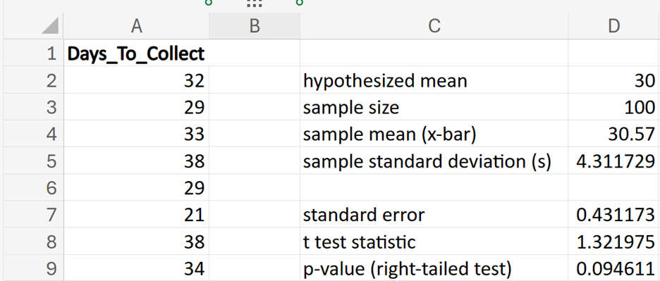
Since the p-value (level of significance), you fail to reject the null hypothesis.

Step 6: Interpret the Results

Since the p-value (0.0946) is greater than the significance level (0.05), you fail to reject the null hypothesis. This means there is not enough evidence to conclude that the mean number of days to collect accounts receivable is greater than 30 days.

try it

You are working as a data analyst for an insurance company. The company wants to ensure that the average claim amount for a specific type of insurance policy does not exceed $5,000 for all their policies. They collect a sample of claim amounts (in dollars) for recent claims to test if the average claim amount for all their policies has exceeded this threshold.

Using the data in the claim_amounts.xlsx Excel file, perform a hypothesis test to determine if the average claim amount for these policies exceeds $5,000. Use a level of significance of 0.05. Interpret the results of the hypothesis test.

Solution:



Null and alternative hypotheses:

• H₀:
• H₁:

Using Excel, you find the p-value for this test to be 0.0129. The Excel worksheets with the values of the test statistic and p-value are provided below.



Interpretation: Since the p-value (0.0129) is less than the significance level (0.05), you reject the null hypothesis. Based on the sample of claim amounts, you have evidence to conclude that the average claim amount for all claims for the insurance company is more than $5,000.

watch

Follow along with this video on performing a right-tailed hypothesis test on average claim amount.

1d. Left-Tailed Hypothesis Test for a Mean

Let’s walk through a practical example of a left-tailed hypothesis test for a mean.

EXAMPLE

GreenTech Solutions, a leading company in sustainable technology, recently implemented a new expense tracking system aimed at reducing operating costs. The CFO (Chief Financial Officer) is keen to evaluate whether this new system has effectively decreased the average monthly operating costs, which were previously $200,000. To assess the impact, the CFO has decided to conduct a hypothesis test.

As a business data analyst, you have been tasked with analyzing the monthly operating costs data to determine if the implementation of the new expense tracking system has significantly decreased the average monthly operating costs from the previous average of $200,000.

In performing this hypothesis test, you will complete the following steps.

Step 1: State the Hypotheses

• H₀:
• H₁:

Step 2: Gather the Data

In Excel, you have a sample of 100 months of operating costs. Using the data in Excel, you find:

• 
• 
• 

Step 3: Choose a Significance Level

Use a level of significance,

Step 4: Perform a Statistical Test

Once again, since σ is not known, you will use the t-test to conduct this test. The test statistic is given by where μ₀ is the hypothesized mean in the null hypothesis, $200,000 in this example.

A test statistic of -1.71 means that the sample mean is 1.71 standard deviations below the hypothesized population mean.

You use the t-distribution to find the p-value for the left-tailed hypothesis test. The graph below shows the t-distribution for a left-tailed hypothesis test. The orange dashed line at shows the observed test statistic. The orange shaded area represents the p-value, indicating the probability of observing the test statistic or something more extreme if the null hypothesis is true.



In a left-tailed test, you look for extreme values to the left end of the distribution, because you want to see if the sample mean is significantly less than the hypothesized mean.

You will now use Excel to find the p-value for this left-tailed hypothesis test. Using the data in the monthly_operating costs.xlsx file, perform the following.

For guidance, the Excel formulas are shown in the screenshot below.



1. In cell C2, enter hypothesized mean. In cell D2, enter 200000.

2. In cell C3, enter sample size. In cell D3, enter 100.

3. In cell C4, enter sample mean (x-bar). In cell D4, enter the following formula:

=AVERAGE(A2:A101)

4. In cell C5, enter sample standard deviation (s). In cell D5, enter the following formula:

=STDEV.S(A2:A101)

5. In cell C7, enter standard error. In cell D7, enter the following formula:

=D5/SQRT(D3)

6. In cell C8, enter t test statistic. In cell D8, enter the following formula:

=(D4-D2)/D7

7. In cell C9, enter p-value (right-tailed test). In cell D9, enter the following formula:

=T.DIST(D8,99,TRUE)

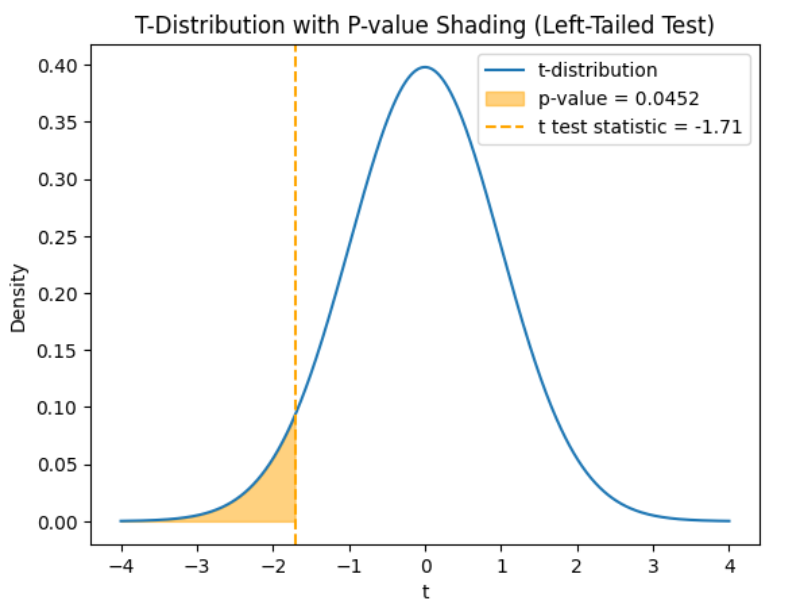
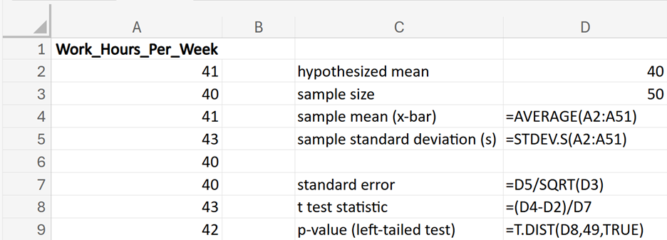
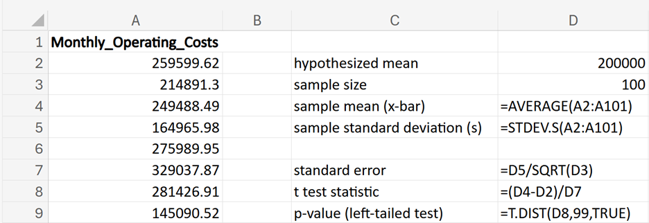
The T.DIST() Excel function is used to calculate the p-value for this left-tailed test. The first argument is the value of the test statistic and the second argument is the degrees of freedom for the t-distribution, which is The third argument is a logical value that specifies to calculate the cumulative probability up to the test statistic, which is the left-tailed p-value for the t-distribution.



Step 5: Make a Decision

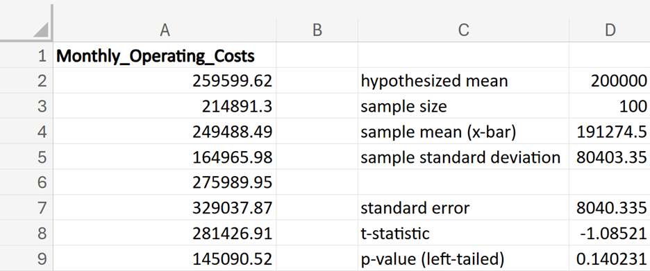
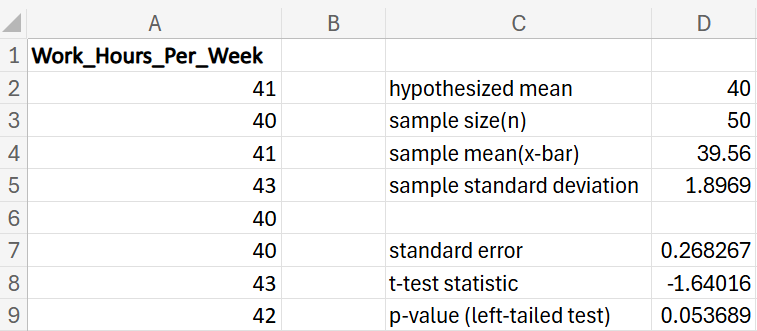
Since the p-value (level of significance), you reject the null hypothesis.

Step 6: Interpret the Results

Since the p-value (0.0452) is less than the significance level (0.05), you reject the null hypothesis. This means there is enough evidence to conclude that the mean operating cost is less than $200,000.

try it

You are a data analyst at a company that is concerned about employee work-life balance. The company believes that employees should work an average of 40 hours per week. To ensure this, you have collected data on the number of hours worked per week by 50 employees. You want to test if the average work hours per week is less than 40 hours for all employees.

Using the data in the employee_work_hours.xlsx Excel file, perform a hypothesis test to test if the average number of hours worked for this sample of employees is less than 40 hours per week. Use a level of significance of 0.05. Interpret the results of the hypothesis test.

Solution:



Null and alternative hypotheses:

• H₀:
• H₁:

Using Excel, you find the p-value for this test to be 0.0765. The Excel worksheets with the values of the test statistic and p-value are provided below.



Interpretation: Since the p-value (0.0765) is less than the significance level (0.05), you fail to reject the null hypothesis. There is not enough statistical evidence to conclude that the average work hours per week for all employees is less than 40 hours.

watch

Check out this video on performing a left-tailed hypothesis test on the average amount of hours worked.