Nonlinear and Non-Smooth Optimization Models

1. Nonlinear Optimization Models

The sections below will guide you through a basic understanding of the concepts and applications of nonlinear optimization models in business data analytics.

1a. Definition

In a previous tutorial, you were introduced to the concept of nonlinear programming. To recap, nonlinear programming involves optimization problems where the objective function or any of the constraints are nonlinear. This means that the relationships between the decision variables are not straightforward or proportional, as they are in linear programming.

Nonlinear optimization deals with problems where the objective function or constraints can involve quadratic, cubic, exponential, or logarithmic terms. These nonlinear relationships allow for a broader range of real-world applications but also make the problems more challenging to solve. Unlike linear optimization, where the objective function and constraints form straight lines, nonlinear optimization involves curves and more complex shapes.

For example, consider a company that wants to maximize customer satisfaction based on the number of products A and B produced. Suppose customer satisfaction increases with the number of products but at a decreasing rate due to market saturation. The objective function might look like this:

Maximize:

Nonlinear optimization models are essential in business data analytics because they can accurately represent complex real-world scenarios. By understanding and applying nonlinear optimization, businesses can make more informed decisions that consider the complex relationships between variables, leading to better outcomes and improved efficiency.

1b. Importance in Decision-Making for Business Data Analytics

In the world of business, making the right decisions can be the difference between success and failure. Businesses often face complex problems that involve multiple factors and constraints. Linear optimization models, which assume straightforward and proportional relationships between variables, are useful for many scenarios. However, more complex business situations involve nonlinear relationships. This is where nonlinear optimization models come into play.

While linear programming is important, many real-world situations are not linear. The relationships between variables can be more complex and involve curves or other nonlinear patterns. Here are a few reasons why nonlinear optimization models are important:

Realistic Modeling of Complex Relationships:
In many business situations, the relationship between variables is not linear. For example, the impact of pricing on demand is often nonlinear. As prices increase, demand may decrease, but not in a straight line. Nonlinear optimization models can capture these complex relationships, providing a more accurate representation of the real world.

Handling Diminishing Returns:
Many business processes experience diminishing returns, where the benefit gained from an additional unit of input decreases as the input increases. Nonlinear optimization models can accurately capture this phenomenon, helping businesses avoid over-investing in areas with diminishing returns.

For example, consider the relationship between advertising spend and customer acquisition. Initially, increasing the advertising budget might lead to a significant increase in new customers. However, as the budget continues to grow, the rate of acquiring new customers may start to decrease. This diminishing return on investment is a nonlinear relationship that can be captured by nonlinear optimization models.

Let’s examine an example of when a nonlinear model is required for an optimization problem.

EXAMPLE

You work as a business data analyst for a company that runs ads on various social media platforms like Facebook, Instagram, and X. The goal is to find the best way to allocate the advertising budget across these platforms to get the most customer engagement (likes, shares, comments). However, the relationship between advertising spend and customer engagement is not straightforward. Initially, spending more on ads increases engagement significantly, but after a certain point, the additional engagement gained from spending more starts to decrease.

The objective function represents the total customer engagement based on the advertising spend on each platform. The nonlinear objective function can be described as follows:

Maximize:

where:

• F is the advertising spend on Facebook
• I is the advertising spend on Instagram
• X is the advertising spend on X

Let’s break down the objective function and understand how this objective function incorporates a nonlinear component to the business problem.

• : This part means that for every dollar spent on Facebook ads, the initial engagement increases by 200 units. So, if the company spends $1 on Facebook ads, the engagement from Facebook is 200 units.
• : Similarly, for every dollar spent on Instagram ads, the initial engagement increases by 150 units. So, if the company spends $1 on Instagram ads, the engagement from Instagram is 150 units.
• : For every dollar spent on X ads, the initial engagement increases by 100 units. So, if the company spends $1 on X ads, the engagement from X is 100 units.
• : This part shows that as the advertising spend on Facebook increases, the additional engagement gained from spending more starts to decrease. This is because there is a limit to how much engagement can be gained from additional spending.
• : Similarly, as the advertising spend on Instagram increases, the additional engagement gained from spending more starts to decrease.
• : As the advertising spend on X increases, the additional engagement gained from spending more starts to decrease.

This objective function is nonlinear because it includes squared terms and which create a curved relationship between the advertising spend and the total engagement. As the advertising spend on each platform increases, the additional engagement gained from spending more decreases, illustrating how a nonlinear optimization function can capture the concept of diminishing returns.

2. Non-Smooth Optimization Models

Non-smooth optimization models are important for solving problems where the objective functions have sharp corners, jumps, or sudden changes. Unlike smooth optimization, which deals with continuous and smooth functions, non-smooth optimization handles more complex situations. These models are essential for accurately capturing and optimizing real-world scenarios where things change abruptly. The sections that follow will provide you with a gentle introduction to non-smooth optimization models.

2a. Definition and Simple Example

Non-smooth optimization deals with optimization problems where the functions involved are not smooth. This means that the objective or constraints can have sharp corners, jumps, or discontinuities (breaks in the graph).

In smooth optimization (linear programming, integer linear programming, and nonlinear programming), the objective functions are smooth and continuous, meaning you can draw them without lifting your pencil from the paper. However, in non-smooth optimization, the functions can have abrupt changes and breaks, making them more challenging to work with.

Let’s take a look at an example so you can see an application of a non-smooth optimization problem.

EXAMPLE

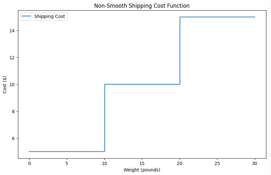
Suppose you work for a company that ships products to customers. The shipping cost depends on the weight of the package. However, the cost does not increase smoothly; instead, it jumps at certain weight limits. Here's how the shipping cost works:

• For packages up to 10 pounds, the cost is $5.
• For packages between 10 and 20 pounds, the cost jumps to $10.
• For packages between 20 and 30 pounds, the cost jumps to $15.

This is a non-smooth function because the cost changes in steps, not smoothly.

Linear Programming Model

Suppose you need to decide how many packages of different weights to ship to minimize the total shipping cost. You have three types of packages:

• Small packages (up to 10 pounds)
• Medium packages (10 to 20 pounds)
• Large packages (20 to 30 pounds)

You want to ship a total of 50 pounds of products. Here's how you can set up the linear programming model:

Objective Function

Minimize the total shipping cost: Minimize:

Decision Variables

• S: Number of small packages
• M: Number of medium packages
• L: Number of large packages

Constraints

The total weight of the packages should be 50 pounds:

The number of packages should be non-negative:

In this example, the shipping cost function is non-smooth because it changes in steps. This makes the optimization problem more challenging, but by using linear programming, you can still find the best way to minimize the total shipping cost while meeting the weight requirement.

You can visualize the non-smooth nature of the objective in the visual below.



In this graph:

• The x-axis represents the weight of the package in pounds.
• The y-axis represents the shipping cost in dollars.

As you can see, the shipping cost changes in steps at certain weight limits (10 pounds and 20 pounds). This creates a non-smooth function with sharp jumps, illustrating how the cost increases abruptly rather than smoothly. This is an example of a non-smooth optimization problem where the function has discontinuities. This means that the graph has points where it suddenly jumps or breaks. In other words, the function is not continuous at those points.

term to know

Non-Smooth Optimization

Optimization problems where the objective function or constraints have abrupt changes or irregularities, making them not smooth or continuous at certain points.

2b. Importance in Decision-Making for Business Data Analytics

Non-smooth models are essential for addressing real-world problems where relationships between variables are not linear or smooth. These models can handle abrupt changes, discontinuities, and other irregular patterns that are common in business environments. Here are a few reasons why non-smooth models are important:

Capturing Realistic Scenarios: In a similar manner to nonlinear models, non-smooth models can optimize objective functions that represent real-world scenarios that are not linear. They can handle scenarios where costs, penalties, or other factors change suddenly, such as bulk discount pricing or penalty fees for late payments. This ability to model real-world complexities makes non-smooth models invaluable for accurate and effective decision-making in business data analytics.

Let’s look at one such example where a non-smooth model can be implemented in a real-world business data analytics scenario.

EXAMPLE

Suppose a company sells office supplies. They offer a bulk discount to encourage larger purchases. If a customer buys fewer than 10 units of a particular item, they pay the regular price of $5 per unit. However, if they buy 10 or more units, they get a discount, and the price drops to $3 per unit. A customer wants to determine the optimal number of units to purchase to minimize the total cost.

The objective is to minimize the total cost. The objective function (cost function) can be defined as follows using a piecewise definition:

where X is the decision v where X is the decision variable representing the number of units to purchase.

Below is a visual of the objective function with the optimal point marked with a green circle.



In this graph, the x-axis represents the number of units purchased, and the y-axis represents the total cost. The green dot shows the best number of units to buy, which is 10 units. This is where the cost is lowest because of the discount.

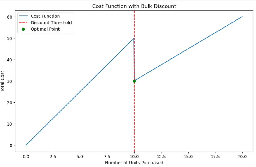
The objective function creates a graph with a sharp change at This sharp change occurs because the cost per unit drops from $5 to $3 when the number of units purchased reaches 10. This sudden change in cost creates a non-smooth function.

In the context of the problem, the cost changes abruptly when the number of units purchased reaches 10. If the customer buys fewer than 10 units, they pay the regular price. But if the customer buys 10 or more units, they receive a discount, and the price drops. This sudden change in cost creates a sharp corner in the graph, making the function non-smooth.

So, the non-smoothness comes from the abrupt change in the cost at the 10-unit mark, which is represented by the sharp corner in the graph.

Improving Decision Accuracy: Non-smooth models help make better decisions by dealing with tricky and unexpected changes in real-world data. They can handle sudden shifts and unusual patterns that smooth models might miss. This means they give more accurate and reliable insights, leading to smarter and more effective business strategies.

Let’s take a look at how a non-smooth optimization model can assist a company in improving decision accuracy.

EXAMPLE

You work for a company that receives a lot of emails every day. Some of these emails are important, but others are spam (unwanted emails). You want to create a system to help decide which emails are spam and which are not.

The goal is to improve the accuracy of the system that classifies emails as "spam" or "not spam." This involves minimizing the errors or penalties for misclassified emails.

To do this, you can use a non-smooth model called the hinge loss function. This function helps you focus on the emails that are most likely to be misclassified, making your system more accurate. The objective function in this optimization problem is to minimize the total loss (or penalty) across all emails.

The hinge loss function is used to calculate the loss for each email based on its prediction score. In plain words, this function means to take the maximum value of 0 and This means that for any value of X, you take the larger value between 0 and

Here's what this function does:

If the prediction score (X) is greater than or equal to 1, the loss is 0. This means the system is confident that the email is not spam.

If the prediction score (X) is less than 1, the loss increases as X decreases. This means the system is less confident or wrong about the email not being spam, and the loss increases.

The prediction score is a value that the system assigns to each email to indicate how confident it is that the email is not spam. Higher scores mean the system is more confident that the email is not spam, while lower scores mean the system is less confident.

• Positive Prediction Scores: A positive prediction score means the system thinks the email is likely not spam. The higher the score, the more confident the system is that the email is not spam.
• Negative Prediction Scores: A negative prediction score means the system thinks the email is likely spam. The lower the score, the more confident the system is that the email is spam.

Below is a visual of the hinge loss system.



In this graph:

• The x-axis represents the prediction score from the system.
• The y-axis represents the loss.

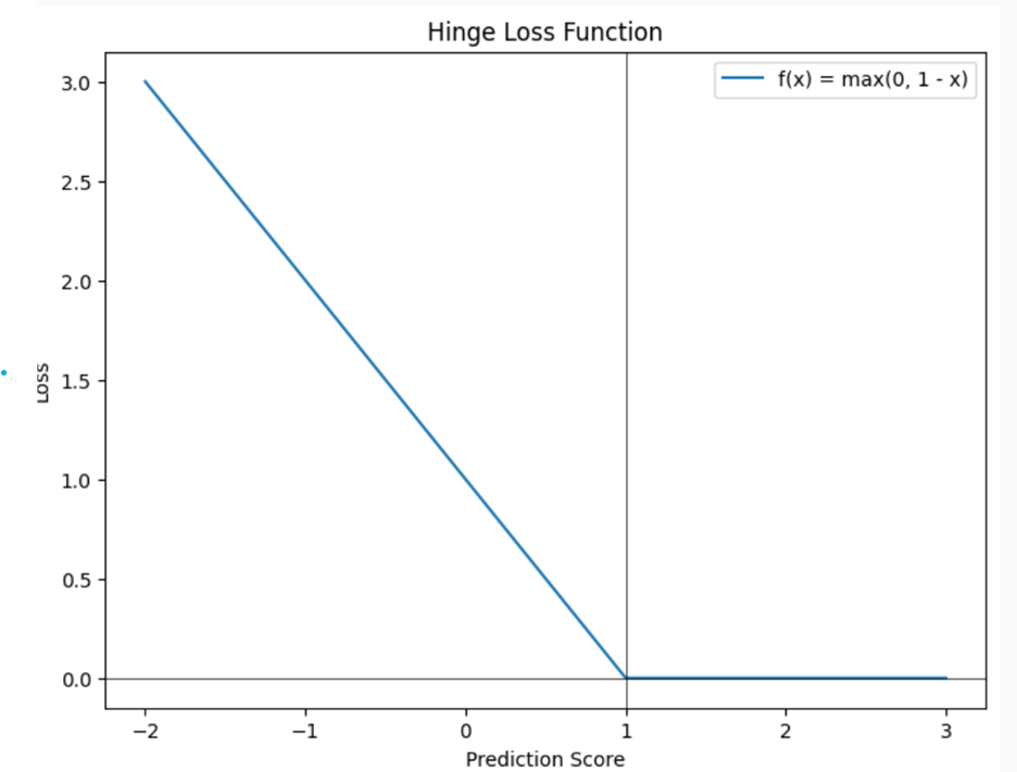
The sharp corner at shows where the function is non-smooth. This corner helps the system focus on misclassified emails, improving its accuracy.

The graph of the hinge loss function has a sharp corner at This corner is where the function changes direction suddenly. In smooth functions, the graph would be curved or straight without any sharp turns.

At the value of the function changes abruptly. For X values greater than or equal to 1, the function value is 0. For X values less than 1, the function value increases as X decreases. This sudden change makes the function non-smooth.