Moving Averages

1. Introduction to Moving Averages

Moving averages are a basic yet powerful tool used in data analytics to understand trends over time. They help smooth out short-term fluctuations in data, making it easier to see the overall pattern. A moving average is a method used to analyze data points by creating a series of averages of different subsets of the full dataset. Imagine you have daily sales data for a store. The sales might go up and down each day, making it hard to see the trend. A moving average helps by averaging the sales over a set number of days, giving you a clearer picture of the trend.

Moving averages are used in many fields to analyze trends and make forecasts. Here are a few examples:

• Stock Market: Investors use moving averages to identify trends in stock prices and make decisions about buying or selling stocks.
• Sales Analysis: Businesses use moving averages to track sales performance over time, helping them make forecasts.
• Website Traffic: Website owners use moving averages to understand trends in visitor numbers, helping them to make decisions about marketing and content strategies.

term to know

Moving Average

An analytical forecasting technique that smooths out time series data by creating a set of averages using different subsets of the data.

1a. Moving Average Calculation and Example

To understand how a simple moving average works, let's break down the calculation process step-by-step and illustrate it with a practical example.

 To calculate a moving average, follow these steps: 

1. Identify the Time Period: Determine the time period for your data points, such as days, weeks, or months. This helps to set the context for your moving average calculation.
2. Choose the Window Size: Decide how many data points you want to include in the average. This is called the window size. For example, a 5-week moving average uses the most recent 5 weeks of data.
3. Calculate the Average (Forecast): Add up the data points in the window and divide by the number of points in the specified window. This gives you the moving average for that period.
4. Move Forward: Shift the window forward by one data point and repeat the calculation.

EXAMPLE

Suppose you have the following daily sales data for a week:

• Day 1: $100
• Day 2: $120
• Day 3: $130
• Day 4: $90
• Day 5: $150
• Day 6: $170
• Day 7: $160

To calculate a 3-day moving average, follow these steps:

Day 3 Forecast: Calculate the average of Day 1, Day 2, and Day 3.

Day 4 Forecast: Move one day forward and calculate the average of Day 2, Day 3, and Day 4.

Day 5 Forecast: Move one day forward and calculate the average of Day 3, Day 4, and Day 5

Day 6 Forecast: Move one day forward and calculate the average of Day 4, Day 5, and Day 6

Day 7 Forecast: Move one day forward and calculate the average of Day 5, Day 6, and Day 7.

The table below shows the actual sales values, and the forecasted values based on the 3-day moving averages.

Day	Sales (Actual Data Values)	3-Day Moving Average Forecasts
Day 1	$100
Day 2	$120
Day 3	$130	$116.67
Day 4	$90	$113.33
Day 5	$150	$123.33
Day 6	$170	$136.67
Day 7	$160	$160.00

With the forecasted values determined, you can calculate forecast accuracy measures, such as MSE, MAE, and MAPE, as covered in the previous tutorial.

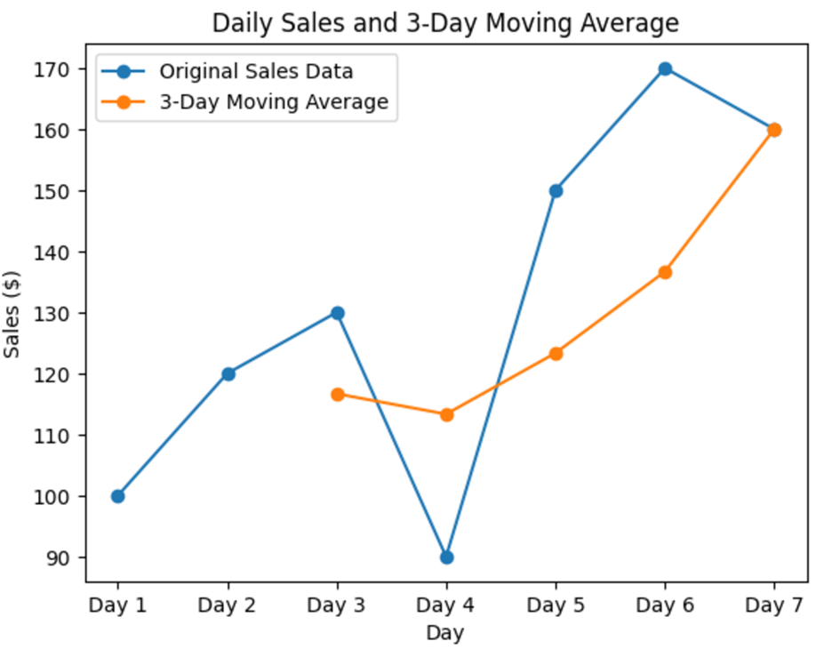
Visualizing the original time series data along with the forecasts can help you understand how moving averages smooth out fluctuations. Below is a plot showing the original sales data and the 3-day moving average forecasts. As you can see, the moving average line is smoother than the original sales data line. This smoothing effect helps to highlight the overall trend by reducing the impact of short-term fluctuations.

The "moving" part of the moving average means that you keep shifting the set of data points you are averaging by one time period at a time (days in the previous example). This helps to smooth out the data and see the trend more clearly. In the previous example, you performed the following:

• First 3 days: You start by averaging the sales of Day 1, Day 2, and Day 3.
• Move forward: Then, you move one day forward and average the sales of Day 2, Day 3, and Day 4.
• Keep moving: You continue this process, moving one day forward each time, until you reach the end of your data.

try it

Suppose you have the following weekly sales data for 10 weeks:

• Week 1: $500
• Week 2: $550
• Week 3: $600
• Week 4: $450
• Week 5: $700
• Week 6: $750
• Week 7: $800
• Week 8: $650
• Week 9: $900
• Week 10: $850

Using the data provided, calculate the 5-week moving average for each week starting from Week 5.

Week	Sales (Actual Data Values)	5-Week Moving Average Forecasts
Week 1	$500
Week 2	$550
Week 3	$600
Week 4	$450
Week 5	$700	$560
Week 6	$750	$610
Week 7	$800	$660
Week 8	$650	$670
Week 9	$900	$760
Week 10	$580	$790

1b. Forecasting with Moving Averages: Applications and Limitations

Moving averages are not just useful for understanding past trends; they are also powerful tools for forecasting future values. By analyzing the smoothed data, you can make more accurate predictions about future trends.

Moving averages are particularly effective for short-term range forecasts, such as predicting the next time period. This is because they smooth out short-term fluctuations and provide a clearer view of the immediate trend. For example, you calculated the 3-day moving average for sales data using the table below. The forecasted sales for Day 8 would be the same as the 3-day moving average for Day 7, which is $160.

It is important to note that moving averages are most suitable for stationary data—data whose statistical properties, such as mean and variance, do not change over time. When your data exhibits considerable trends or seasonality, moving averages are not the best forecasting method.

Below are some limitations of moving averages to consider when deciding whether to use this method for forecasting:

• Trends: If your data shows a long-term upward or downward trend, a simple moving average might lag behind the actual values, as it does not account for the trend's direction.
• Seasonality: For data with seasonal patterns, such as monthly sales that peak during certain times of the year, moving averages can obscure these patterns, leading to inaccurate forecasts.

2. Real-World Application of Moving Averages in Python

In this section, you will explore how moving averages can be applied in a real-world business scenario using Python.

2a. Forecasting with Moving Averages

You are going to step into the shoes of a data analyst and use two different moving average models to forecast monthly sales in the upcoming example.

did you know

The dropna() function in pandas is used to remove missing values (NaNs) from your data. When you apply dropna() to a DataFrame, it returns a new object with the NaN values removed. This is particularly useful when you need to perform calculations or analyses that require complete data. For example, in the code below, dropna() is used to ensure that only valid (non-missing) moving average values are considered for the forecast.

EXAMPLE

Suppose you are a data analyst at TrendyBox, a subscription box service for trendy fashion accessories. Your task is to analyze the monthly sales data over the past two years (2023-2024) and forecast the sales for the next month (January 2025) using moving averages in Python. You can access the GitHub data at:
https://raw.githubusercontent.com/sophiaAcademics/BDA_Excel/main/StudentData/Tutorials/Unit5/5.2.3/trendybox_sales.xlsx

The code below imports pandas, imports an Excel file from a URL, and creates a pandas DataFrame named sales_ma before continuing to calculate moving averages.



Step 1: Calculate 3- and 6-month moving averages

sales_ma['MA_3'] = sales_ma['Sales'].rolling(window=3).mean()

• This line calculates the 3-month moving average by:
  • Accessing the Sales column in the sales_ma DataFrame.
  • Then, it applies a rolling window of size 3 to the Sales column, meaning that for each data value in the column, it considers the current value and the two preceding values.
  • The mean() function calculates the mean (average) of the values within this rolling window, resulting in a 3-month moving average.
  • Finally, the calculated 3-month moving average is stored in a new column MA_3 in the sales_ma DataFrame.

sales_ma['MA_6'] = sales_ma['Sales'].rolling(window=6).mean()

• The line calculates the 6-month moving average in a similar manner as the 3-month moving average to create the MA_6 column. But now the window contains the past 6 sales values when calculating the average.

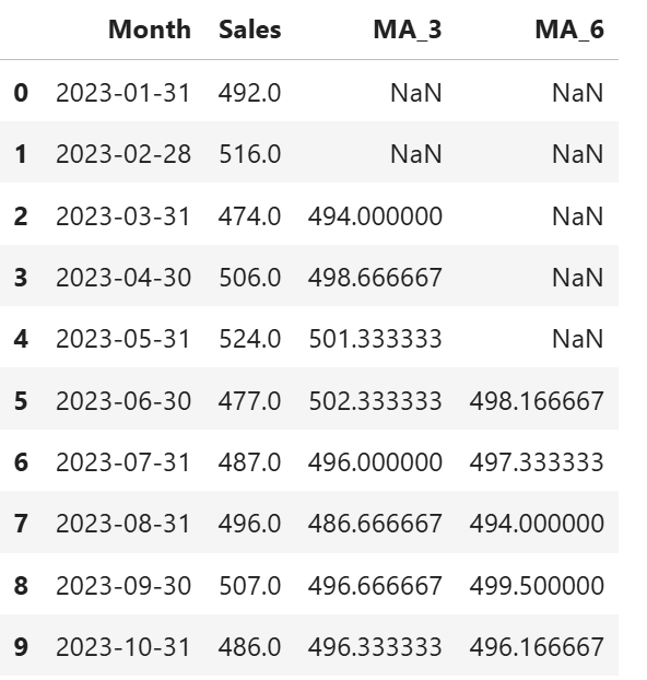
Step 2: View the 3-month and 6-month moving averages for the first 10 sales values.

sales_ma.head(n=10)

This line displays the first 10 rows of the sales_ma DataFrame.

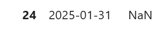
To find missing values, remember we are looking for the following notation, NaN, which is shown in this screenshot. Here, the 25 observations do not have a value:



The 3-month moving average requires three data points to calculate the first average. Therefore, the first two rows will have NaN values in the MA_3 column, because there are not enough preceding data points to compute the average.

Similarly, the 6-month moving average requires six data points to calculate the first average. As a result, the first five rows will have NaN values in the MA_6 column, because there are not enough preceding data points to compute the average.

These missing values are expected behavior.



The code below creates the forecasted sales value for January 2025 using the 3-month and 6-month moving averages.

Step 4: Forecast for January 2025 using the 3-month moving average.

forecast_3 = sales_ma['MA_3'].dropna().iloc[-1]

• This line forecasts the 3-month moving average by:
  • Accessing the MA_3 column in the sales_ma DataFrame, which contains the 3-month moving averages.
  • Then, it applies the dropna() function to remove any NaN values from the MA_3 column. This step is crucial because the moving average calculation can result in NaN (missing) values at the beginning of the column where there are not enough data points to compute the average.
  • Finally, the iloc[-1] function selects the last non-NaN (missing) value in the MA_3 column. This value is used as the forecast for January 2025.

forecast_6 = sales_ma['MA_6'].dropna().iloc[-1]

• Similarly, as with the forecasted 3-month moving average, this line forecasts the 6-month moving average by accessing the MA_6 column, removing any NaN (missing) values, and selecting the last non-NaN (missing) value to use as the forecast for January 2025.

Step 5: Print the 3- and 6- month forecasted values.

print(forecast_3)
print(forecast_6)

• These two lines print the 3- and 6- month forecasted values. The forecast values are shown below.

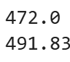
The forecasted sales for January 2025 are $472 using the 3-month moving average and $491.83 using the 6-month moving average.

Now it is your turn to practice forecasting with moving averages in Python on your own!

try it

Suppose you are a data analyst at TechInsights, a tech blog that provides insights and updates on the latest technology trends. Your task is to analyze the monthly website traffic data (number of visitors to the website) over the past year (2024) and forecast the number of visitors for the next month (January 2025) using moving averages in Python.

You can access the GitHub data at:
https://raw.githubusercontent.com/sophiaAcademics/BDA_Excel/main/StudentData/Tutorials/Unit5/5.2.3/TechInsights_website_traffic.xlsx

Perform the following:

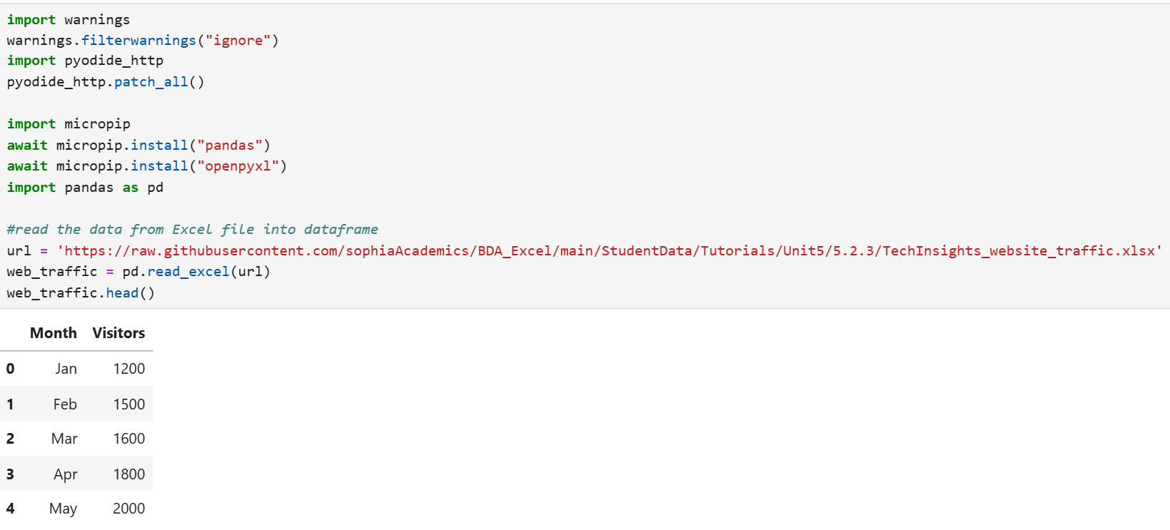
1. Import the Excel file, create a pandas DataFrame named web_traffic_ma, and view the first five rows of the data frame.
2. Create 2- and 4-month moving average forecasts for the number of visitors for the TechInsights blog website. Name the column that will contain the 2-month moving average MA_2, and name the column that will contain the 4-month moving average MA_4. View the first 10 rows of the data to verify a couple of the moving averages and ensure the NaN (missing) values that you observe make logical sense.
3. Forecast the number of visitors for January 2025 using the 2- and 4-month moving averages.

Solution:

1. The code below will create a pandas DataFrame named web_traffic_ma and display the first five rows of the data.



2. The code below creates 2- and 4-month moving averages for the forecasted number of visitors to the TechInsights blog website. The columns MA_2 and MA_4 contain the forecasted values.



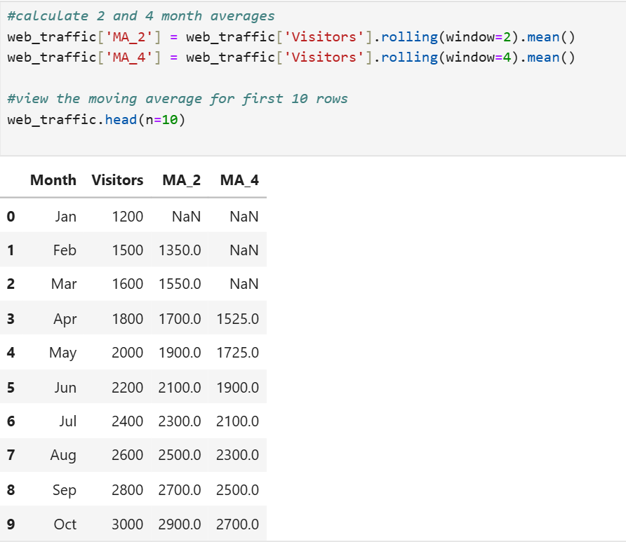
In the output shown above:

• The 2-month moving average (MA_2) has a NaN (missing) value for January, because there is no previous month to average with.
• The 4-month moving average (MA_4) has NaN (missing) values for January, February, and March, because there aren't enough previous months to calculate the average.

These missing values are expected and indicate that the moving average calculation requires a certain number of previous data points to produce a valid result. As more data points become available, the moving averages will be calculated for subsequent months.

3. The code below calculates the forecast for January 2025 using the 2-month and 4-month moving averages, based on the most recent available data.

This code snippet below first drops any NaN (missing) values from the moving average columns to ensure only valid data points are used. Then, it selects the last available value from each moving average column (MA_2 and MA_4) to use as the forecast for January 2025. Finally, it prints the forecasts for both the 2-month and 4-month moving averages.



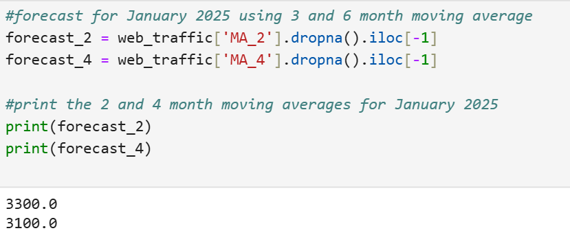
The forecasted number of visitors to the TechInsights blog website for January 2025 using the 2-month moving average is 3,300, and the 4-month moving average forecast is 3,100.

watch

This video looks at TechInsight Blog website visitors and evaluates moving averages to forecast website visits.

2b. Comparing Moving Average Forecasts

In the last section, you built two different moving average forecast models to predict monthly sales. Now, you will compare these forecasts to evaluate their accuracy. By analyzing the performance of each model, you will gain insights into which moving average method provides more reliable predictions for TrendyBox's sales data.

This comparison will involve calculating and interpreting key error metrics, such as Mean Squared Error (MSE), Mean Absolute Error (MAE), and Mean Absolute Percentage Error (MAPE). Let's dive into the details and see how these models stack up against each other.

EXAMPLE

Returning to the TrendyBox monthly sales data (https://raw.githubusercontent.com/sophiaAcademics/BDA_Excel/main/StudentData/Tutorials/Unit5/5.2.3/trendybox_sales.xlsx), you will now compare the forecast accuracy of the two moving average forecast methods you constructed earlier. You are going to evaluate the forecast of each forecast method using MSE, MAE, and MAPE. Round each of the forecast measures to one decimal place.

The code below imports pandas, imports an Excel file from a URL, and creates a pandas DataFrame named sales_ma.



Let’s break down the new code line by line.

Step 1: Prepare the data for the forecast accuracy measures calculations.

sales_ma.dropna(inplace=True)

• This line removes any rows from the sales_ma DataFrame that contain NaN (missing) values in any column. This ensures that the subsequent calculations for MSE, MAE, and MAPE are performed on complete data without missing values.
• The argument inplace=True in the code means that the operation will be performed directly on the sales_ma DataFrame, modifying it in place without creating a new DataFrame.

In the previous tutorial, detailed explanations for the forecast accuracy measures in Python were provided. The following code for computing MSE, MAE, and MAPE is the same as used in the previous tutorial, but with different column names. A brief summary of the code will be provided, since the detailed explanations have already been covered.

Step 2: Calculate MSE for the 3- and 6-month moving average forecasts.

#calculate and print the Mean Square Error (MSE) for 3-month MA
mse_3 = ((sales_ma['Sales'] - sales_ma['MA_3']) ** 2).mean()
print(f"The Mean Square Error (MSE) for 3-month MA is: {mse_3: .1f}")

#calculate and print the Mean Square Error (MSE) for 6-month MA
mse_6 = ((sales_ma['Sales'] - sales_ma['MA_6']) ** 2).mean()
print(f"The Mean Square Error (MSE) for 6-month MA is: {mse_6: .1f}")

• These lines calculate MSE for the 3- and 6-month moving averages by squaring the errors (differences between actual sales and the 3- and 6-month moving averages, which contain the forecasted values), taking the mean of these squared errors, and printing the result.
  
  The Sales column contains the actual value of the sales for each month and the columns MA_3 and MA_6 contain the forecasted values for the 3- and 6-month moving averages, respectively.

The MSE for the 3- and 6-month moving average forecasts are shown below.



The output tells you that the 3-month moving average provides a more accurate forecast than the 6-month moving average. This is indicated by the lower Mean Square Error (MSE) value for the 3-month moving average (305.3) compared to the 6-month moving average (396.4).

Step 3: Calculate MAE for the 3- and 6-month moving average forecasts.

#calculate and print the Mean Absolute Error (MAE) for 3-month MA
mae_3 = (sales_ma['Sales'] - sales_ma['MA_3']).abs().mean()
print(f"The Mean Absolute Error (MAE) for 3-month MA is: {mae_3: .1f}")

#calculate and print the Mean Absolute Error (MAE) for 6-month MA
mae_6 = (sales_ma['Sales'] - sales_ma['MA_6']).abs().mean()
print(f"The Mean Absolute Error (MAE) for 6-month MA is: {mae_6: .1f}")

• These lines calculate the MAE for the 3- and 6-month moving average by taking the absolute value of the errors (differences between actual sales and the 3- and 6-month moving averages, which contain the forecasted values), calculating the mean of these absolute errors, and printing the result.

The MAE for the 3- and 6-month moving average forecasts are shown below.



The output tells you that the 3-month moving average provides a slightly more accurate forecast than the 6-month moving average. This is indicated by the lower Mean Absolute Error (MAE) value for the 3-month moving average (14.4) compared to the 6-month moving average (15.4).

Step 4: Calculate MAPE for the 3- and 6-month moving average forecasts.

#calculate and print the Mean Absolute Percentage Error (MAPE) for 3-month MA
mape_3 = (abs(sales_ma['Sales'] - sales_ma['MA_3']) / sales_ma['Sales']).mean() * 100
print(f"The Mean Absolute Percentage Error (MAPE) for 3-month MA is {mape_3: .1f}%")

#calculate and print the Mean Absolute Percentage Error (MAPE) for 6-month MA
mape_6 = (abs(sales_ma['Sales'] - sales_ma['MA_6']) / sales_ma['Sales']).mean() * 100
print(f"The Mean Absolute Percentage Error (MAPE) for 6-month MA is {mape_6: .1f}%")

• These line calculate the MAPE for the 3- and 6-month moving averages by taking the absolute value of the errors (differences between actual sales and the 3- and 6-month moving averages, which contain the forecasted values), dividing by the actual sales to get the percentage error, calculating the mean of these percentage errors, and printing the result.

The MAPE for the 3- and 6-month moving average forecasts are shown below.



The output tells you that the 3-month moving average provides a more accurate forecast than the 6-month moving average in this context. This is indicated by the lower Mean Absolute Percentage Error (MAPE) value for the 3-month moving average (2.9%) compared to the 6-month moving average (3.2%).

The following table summarizes the forecast accuracy measures you have developed in Python.

Metric	3-Month Moving Average	6-Month Moving Average
MSE	305.3	396.4
MAE	14.4	15.4
MAPE	2.9%	3.2%

The findings from your forecast accuracy analysis show the 3-month moving average consistently shows lower error metrics (MSE, MAE, and MAPE) compared to the 6-month moving average.

This indicates that the 3-month moving average is more responsive to recent changes in the sales data and provides more accurate forecasts for TrendyBox. Therefore, using the 3-month moving average for forecasting would likely result in better inventory management, financial planning, and overall decision-making for the company.

try it

You are going to return to an example you have worked with previously using:
https://raw.githubusercontent.com/sophiaAcademics/BDA_Excel/main/StudentData/Tutorials/Unit5/5.2.3/TechInsights_website_traffic.xlsx

You are a data analyst at TechInsights, a tech blog that provides insights and updates on the latest technology trends. In a previous exercise, you forecasted the number of website visitors for January 2025 using 2- and 4-month moving averages. You will need to return to that code. You are going to assess which moving average is the most accurate. You are going to calculate three forecast accuracy measures, MSE, MAE, and MAPE, for the 2- and 4-month moving averages.

Perform the following.

1. Calculate the three forecast accuracy measures, MSE, MAE, and MAPE, and fill out the table below with your results. Round the forecast accuracy measures to zero decimal places.

Metric	2-Month Moving Average	4-Month Moving Average
MSE
MAE
MAPE

2. Which moving average would you suggest TechInsights use as their forecasted number of visitors for January 2025, based on the forecast accuracy measures?

Solution:

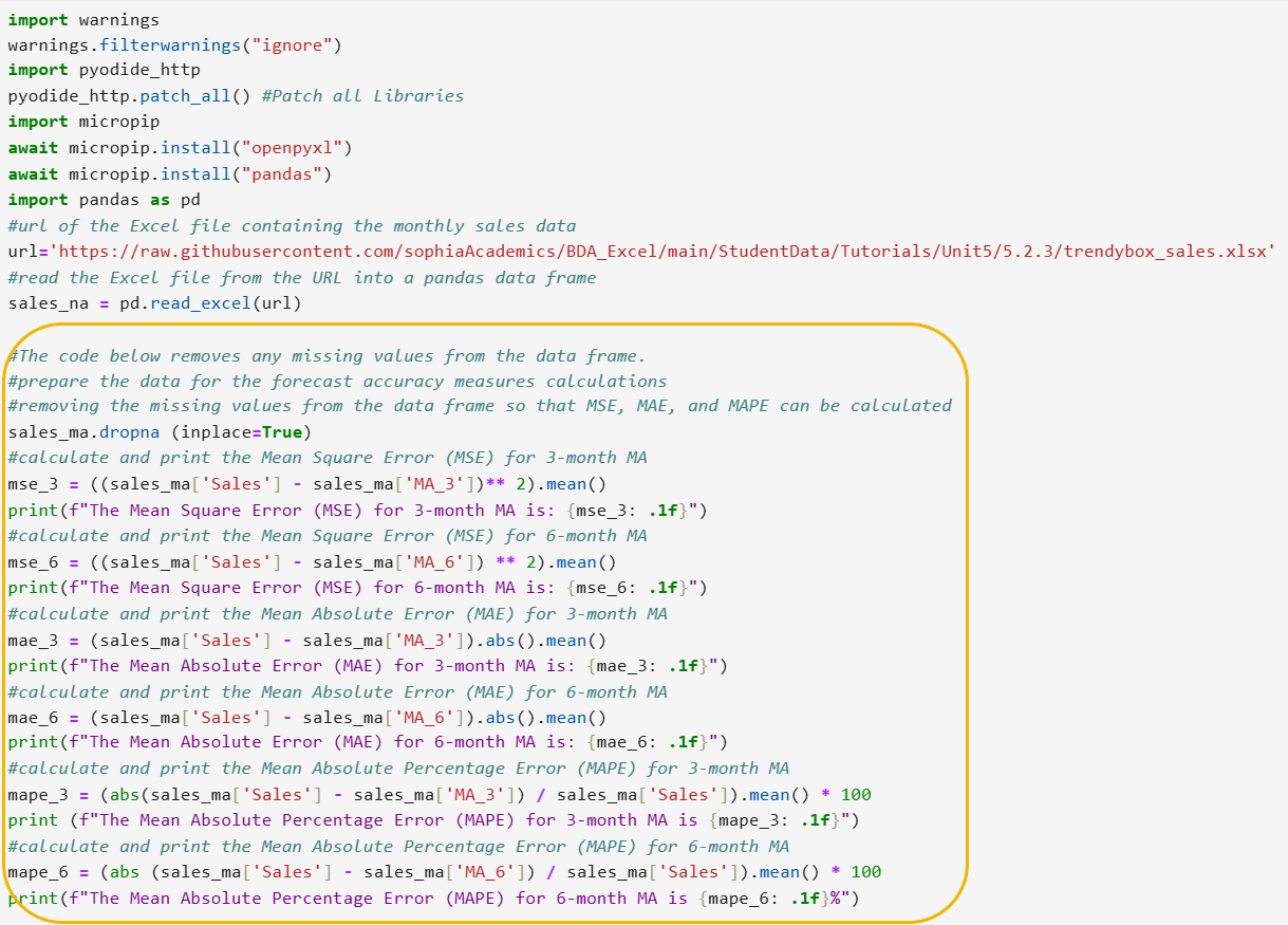
1. The code below will calculate the three forecast accuracy measures, MSE, MAE, and MAPE, for the 2- and 4-month moving averages.



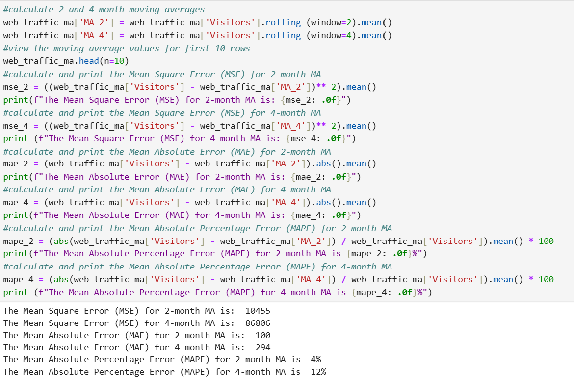
Using the output, fill in the values for the table below.

Metric	2-Month Moving Average	4-Month Moving Average
MSE	10,455	86,806
MAE	100	294
MAPE	4%	12%

2. The 2-month moving average is recommended for forecasting January 2025 visitors because it has lower MSE, MAE, and MAPE values compared to the 4-month moving average, indicating better forecast accuracy.

watch

This video looks at MSE, MAE, and MAPE for the 2- and 4-month moving averages for TechInsight website traffic.

If you noticed in both the example and the exercise for selecting the best moving average, both times the shorter moving average produced the best accuracy. This outcome can be attributed to several factors inherent to shorter moving averages:

1. Sensitivity to Recent Data: Shorter moving averages, such as the 2-month moving average, are more responsive to recent changes in the data. They quickly adapt to the latest trends and fluctuations, providing a more accurate reflection of the current state. This is particularly beneficial in dynamic environments where conditions can change rapidly.
2. Reduced Lag: A shorter moving average has less lag compared to a longer one. This means it can adjust more swiftly to new data points, reducing the delay in capturing the latest trends. This timeliness can lead to more accurate forecasts, especially when recent data is more indicative of future patterns.
3. Minimizing the Impact of Older Data: By focusing on a shorter period, the moving average minimizes the influence of older data, which might not be as relevant to current conditions. This can be crucial in scenarios where the most recent data points are more reflective of future behavior.
4. Adaptability to Seasonal Changes: In cases where there are seasonal or cyclical patterns, a shorter moving average can adapt more quickly to these changes. This adaptability ensures that the forecast remains relevant and accurate, even in the face of seasonal variations.

In conclusion, the choice of moving average window should be based on the specific context and the nature of the data being analyzed. While shorter moving averages often provide better accuracy due to their responsiveness and reduced lag, it's essential to balance this with the potential for increased volatility. By understanding these dynamics, you can make more informed decisions about which moving average to use for forecasting in various scenarios.