Table of Contents |
Imperfect competition in labor markets occurs on the demand side when employers of labor exercise market power. In markets where buyers of labor exercise power, the market is characterized as a monopsony. How is wage and employment determined in this type of labor market, where the employers have market power? How do competitive and monopsonistic market outcomes differ?
Suppose there is only one employer in a labor market. Because that employer has no direct competition in hiring, if they offer wages lower than would exist in a competitive market, employees have few options. If workers want a job, they must accept the offered wage rate. Since the employer is exploiting its market power, we call the firm a monopsonist. A classic example of a monopsony labor market is a remote coal mining town in the Appalachia region. If local coal miners want to work, they must accept the wage rate of the coal company.
How does market power by an employer affect labor market outcomes? Does it make sense that wages will be lower than in a competitive labor market? Let’s explore these questions.
First, we must understand that a monopsonist is the sole employer of labor in a particular market. The monopsonist firm is the labor market. Its impact is similar to a monopoly in the product markets.
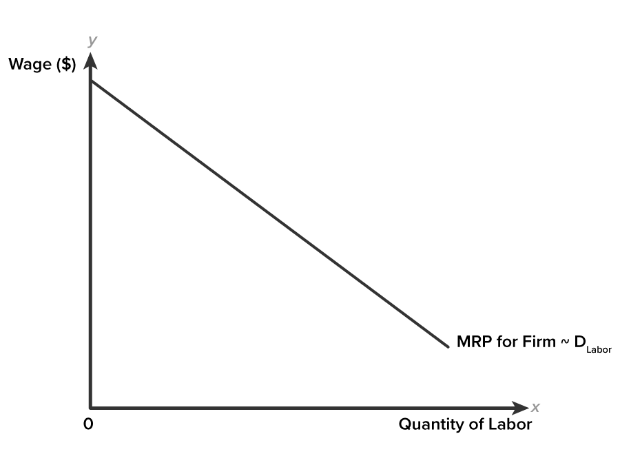
Second, recall that a firm’s demand for labor is the downward-sloping portion of its marginal revenue product (MRP) curve, which represents the additional revenue a firm expects to earn from hiring an additional worker. We calculate MRP by multiplying the MPL by marginal revenue (MR), which is the added revenue from selling an additional unit of product.

Third, now that we understand the firm’s demand for labor curve, let’s identify the supply of labor curve.
Think back to what you learned about the monopoly market structure in the challenge about market environments. Because the monopolist is the sole supplier of a product in the market, it sets its price to profit-maximize. The bad news is that if the monopoly wants to sell a greater quantity of its product, it must lower the price it charges. The monopolist’s demand curve for its product is downward sloping. It obeys the law of demand. Quantity demanded increases as price decreases, holding all else constant.
The monopsonist in the labor market has a similar experience. Because the monopsonist is the sole employer in a labor market, it is a wage setter. However, because a monopsonist faces an upward-sloping market labor supply curve, if the firm wants to hire more workers, the firm must raise the wage rate to market equilibrium. This is in accordance with the law of supply. Quantity supplied increases as price increases, holding all else constant. This creates a dilemma for the monopsonist.
Let’s assume that the monopsonist's only input is labor. Therefore its only production cost is labor cost. The monopsonist determines how many workers to hire in total, rather than sequentially, or one-by-one. This allows us to calculate the wage bill, or total factor cost (TFC) for a given number of workers.
In the table below, the first column represents the number of workers and the second column represents the wage per hour. Notice that the wage rate rises as more workers are hired. Again, this is the law of supply at work. If the firm hires four workers then those workers will each be paid $4 per hour. The third column is total factor cost (TFC) calculated as (Quantity of Labor * Wage per Hour). As more workers are hired, the wage bill, TFC, rises. The final column represents the additional cost of hiring one more worker known as marginal factor cost of labor (MFC).
|
Quantity of Labor (Q) |
Wage per Hour |
Total Factor Cost (TFC = Q * Wage) |
Marginal Factor Cost (MFC) |
|---|---|---|---|
| 1 | $1 per hour | $1 | $1 |
| 2 | $2 per hour | $4 | $3 |
| 3 | $3 per hour | $9 | $5 |
| 4 | $4 per hour | $16 | $7 |
| 5 | $5 per hour | $25 | $9 |
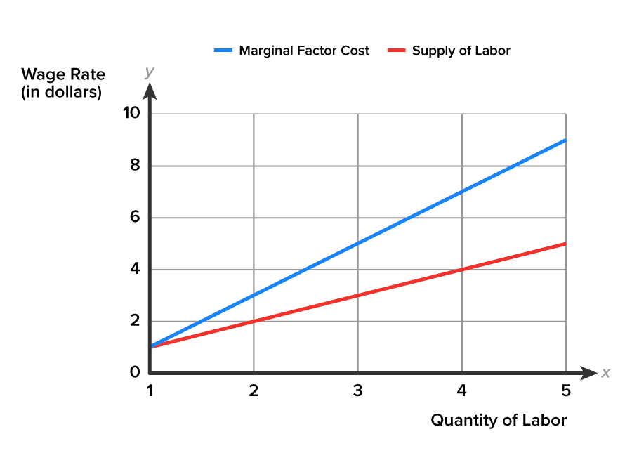
Using the information in the table above, we can create a graph of the supply side of the monopsonist’s labor market.

There are a couple of interesting observations to make about a monopsonist’s labor market.
First, the blue marginal factor cost (MFC) curve illustrates the additional cost of hiring one additional worker, and it increases faster than the red supply of labor curve. In fact, the marginal factor cost of hiring an additional worker (beyond the first worker) is always greater than the wage necessary to pay the additional worker. This is shown as the difference between MFC and supply curve at each quantity of labor.
Why is this the case?
Monopsonies are the sole demander of labor in a particular market, and face the same labor supply curve that all other firms seeking to hire workers face. Hiring another worker from the labor pool is a move up along the supply curve to a higher wage per hour in accordance with the law of supply. At a higher wage rate the quantity of labor supplied is higher. All workers will be paid this market equilibrium wage. The monopsonist compensates all workers at the new wage rate, making up any difference in pay. As a result, the marginal factor cost of hiring an additional worker is greater than the wage paid for an additional worker for any level of employment (above the first worker). Therefore, MFC is above the market supply of labor.
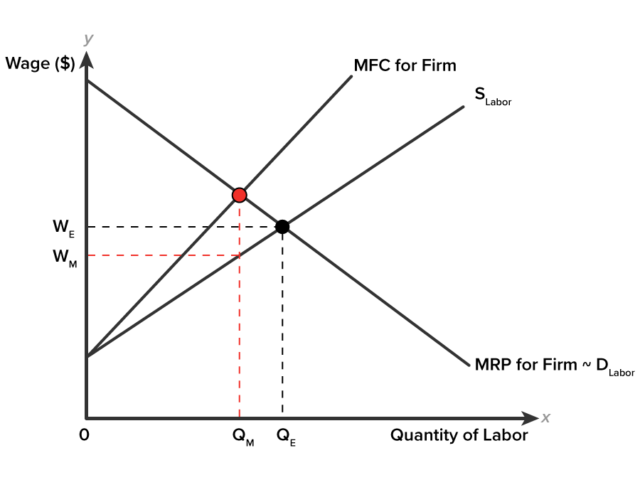
Second, If the firm wants to maximize profits, it will hire the quantity of labor found where the firm’s demand for labor (MRP) intersects with MFC, the additional cost of hiring one more worker. The margins are equal at MRP=MFC. The additional revenue a firm expects to earn from selling an additional worker’s output is equal to the added cost of hiring that additional worker.
The supply curve for labor shows the wage the firm will have to pay to attract a particular quantity of workers. This is depicted in the graph below.
 ).
).  to the point where it meets the supply of labor curve, then read across the red dashed horizontal line to the monopsonist’s wage
  on the vertical axis to the left.
  workers, and will pay each worker the same rate of
  . These workers (
 ) are willing and able to supply labor services at the monopsonist’s wage (
 ).
). workers, and will pay each worker the same wage rate
  given along the labor supply curve.

How does the monopsonist outcome compare to what would occur in a perfectly competitive market? To explore this question, let’s examine the graph you just reviewed in the previous section, but this time in the context of comparing perfectly competitive outcomes to monopsonist outcomes.
Notice in the graph below that in a competitive labor market, wage rate and the number of workers with jobs is determined at the intersection of supply and demand curves. The labor market would clear at  , with quantity demanded equal to the quantity supplied. All workers would be paid the same wage rate of
  .
.
Compared to the competitive outcome, monopsony employers with market power hire fewer workers,  <
<  , and pay lower wage rates,
  <
<  . While pure monopsony may be rare, many employers have some degree of market power in labor markets. The price and quantity outcomes for those employers will be similar to those of a monopsony.

 ) and pay less (
 ) than a firm in a competitive environment (
 and
and  ).
).
 ) line. In Comparison of Market Outcomes you learned that workers seeking employment in a monopsony labor market are paid less and that fewer workers are hired in comparison to a competitive labor market.
Source: THIS TUTORIAL HAS BEEN ADAPTED FROM OPENSTAX “PRINCIPLES OF ECONOMICS 2E”. ACCESS FOR FREE AT https://openstax.org/books/principles-economics-2e/pages/1-introduction. LICENSE: CC ATTRIBUTION 4.0 INTERNATIONAL.