Table of Contents |
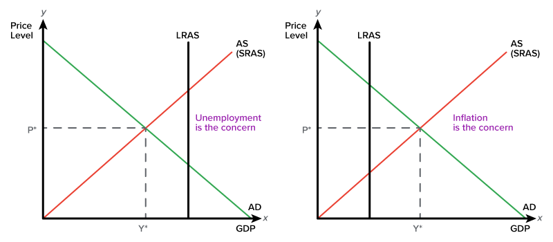
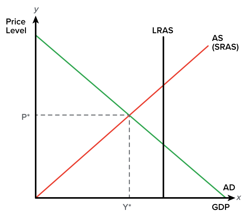
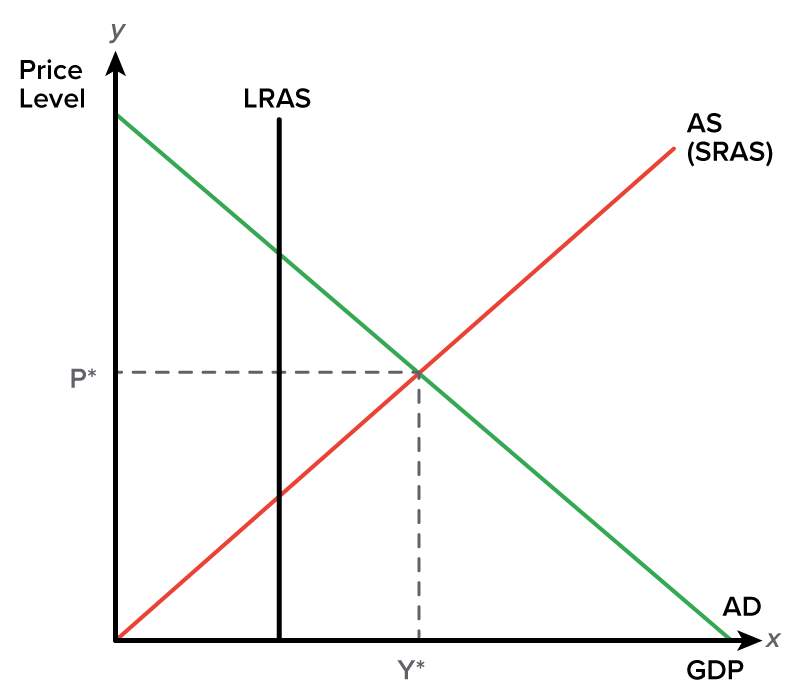
The following two graphs show two different situations where the economy is not in equilibrium. At equilibrium, the long-run aggregate supply (LRAS) curve intersects the point where the short-run aggregate supply (SRAS) and aggregate demand intersect.
At times, our economy produces below full employment, as shown on the left. In this case, there are unemployed resources, and unemployment is a concern.
It is also possible for the economy to produce beyond full employment in the short term, illustrated on the right. In this case, inflation can become a major concern.
In either case, intervention is often needed in the form of action from the government or the Federal Reserve.
When the government intervenes, it sets what is called fiscal policy, which is policy typically set by a central government authority, whereby government spending and taxation are adjusted to stabilize economic activity.
The government has two tools:
These are the three tools of monetary policy:
Expansionary policy is either monetary or fiscal policy that is enacted to stimulate economic growth as measured by the GDP growth rate.
So, why do we want to enact expansionary policy? Well, we do this when unemployment is the concern or when we are producing below full employment.
Here is a chart outlining the tools used by both types of policy to expand the economy.
| Expansionary Policy | |
|---|---|
| Monetary | Fiscal |
| Increase the money supply/entice banks to make loans | Encourage job creation and more spending in the economy |
|
1. Lower the RRR 2. Lower interest rates 3. Buy securities |
1. Increase government spending 2. Cut taxes |
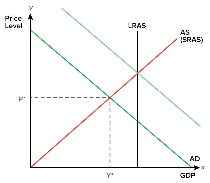
Fiscal policy, as mentioned, directly attempts to create demand by spending money to develop programs, jobs, and so on.
Monetary policy works by increasing the money supply and encouraging people to spend money and take out loans.
Either way, the end result is an increase in aggregate demand, as you can see below, taking the economy to full employment, reducing the unemployment rate, and utilizing all of the resources.
Either fiscal or monetary policy will have a multiplier effect, which is the sum total impact of a policy action on the economy.
The money multiplier is equal to the ratio of the reserve requirement, which is 1 divided by R, where R is the reserve requirement, such that a given reserve requirement will result in a net multiple of the original increase, where we have to multiply by the change in loanable funds.

So, if a bank can make one more loan as a result of a policy, this will create more loans.
With fiscal policy, if even one more person receives a paycheck as a result of a new government program, that person will spend money in businesses. This impacts other people, who then go out and spend more money and so forth.
You can imagine how much more this multiplies on a larger scale in the overall economy whenever expansionary policy is implemented.
This is a situation where policymakers use “excessive fiscal or monetary policies” to get the economy back to equilibrium.
What happens if we stimulate aggregate demand too much with expansionary policy? Well, if the impact on aggregate demand is too much, it can actually push equilibrium temporarily past the LRAS curve.
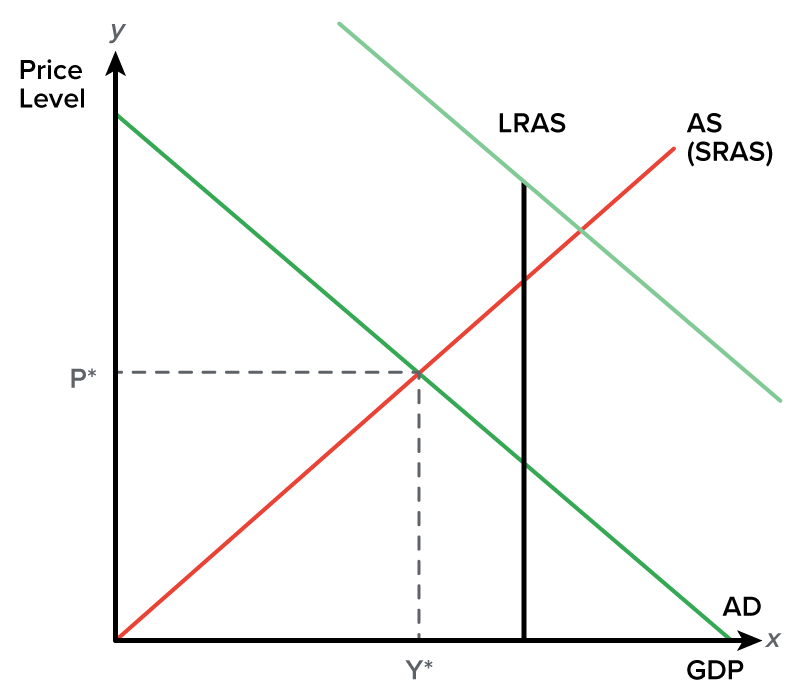
When that happens, notice how prices go up—and the prices going up include input prices.
When suppliers or producers experience increased prices, the SRAS can shift to the left, bringing the economy back to equilibrium, but now at higher prices.
The end result would be an increase in prices or inflation.
It is important to understand that these policies can be used to stimulate aggregate demand to stabilize the economy and move it toward equilibrium. However, overstimulating aggregate demand will not achieve long-run economic growth. Remember that the LRAS curve represents our economy’s ability to produce when all resources are utilized. Unless resources change to shift this curve, we will only create inflation by overstimulating aggregate demand beyond the LRAS.
Now, let’s look at the opposite situation where inflation is the concern. In this case, the government or the Fed needs to slow down the economy through contractionary policy, which is either monetary or fiscal policy that is enacted to slow economic growth, as measured by the GDP growth rate.
| Contractionary Policy | |
|---|---|
| Monetary | Fiscal |
| Decrease the money supply/entice people to keep money in banks | Encourage less spending in the economy |
|
1. Raise the RRR 2. Raise interest rates 3. Sell securities |
1. Decrease government spending 2. Raise taxes |
Fiscal policy decreases demand by cutting spending, while monetary policy works by decreasing the money supply, again encouraging people to save money and take out fewer loans.
Either way, the end result is a decrease in aggregate demand.
As you have seen in these graphs, theoretically, there is a direct relationship between real GDP growth and the price level.
As aggregate demand is stimulated and increases, the economy grows and unemployment falls, pushing prices up.
As aggregate demand decreases, the economy contracts. By decreasing aggregate demand, the attempt is to push prices down. The trade-off is increased unemployment.
This is what the Phillips curve illustrates. It is a graphical depiction of this inverse relationship between inflation and unemployment. Intuitively, higher employment or lower unemployment is consistent with a strong economy and demand. As demand increases beyond short-run supply capabilities or resource constraints, inflation begins to increase.
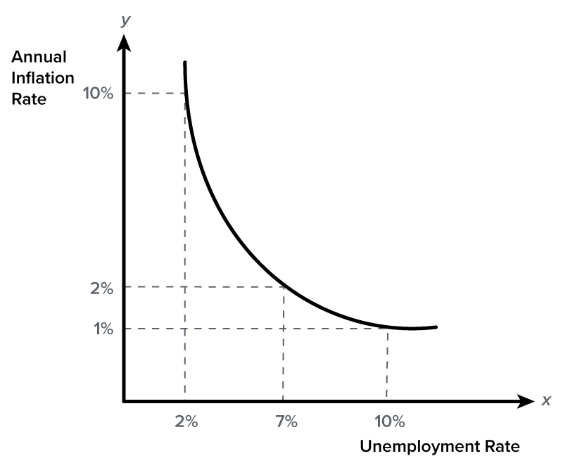
You can see the axes are annual inflation rate and unemployment rate. There is a trade-off between the two because they are inversely related.
When unemployment is low, we tend to have high inflation because of high demand. When unemployment rises, we have lower inflation.
Since inflation is not the concern, the government or Fed can enact some type of expansionary policy, which will lower unemployment. However, there will be a slight increase in prices or inflation.
Now, if inflation exceeds 10%, which is extremely high, the government or the Fed can enact contractionary policy, since employment is significantly below full employment.
There could be lower inflation, but the trade-off is a slightly higher unemployment rate as demand in the economy starts to fall.
Very low levels of unemployment (less than 5%) are generally unsustainable and can create bubbles, such as the housing bubble in the early 2000s. In this case, the government or the Fed will want to cool down the economy by enacting contractionary policies.
Critics of this model sometimes point to the 1970s, when our economy experienced very high rates of inflation at the same time as high unemployment. This is known as stagflation.
We would not be able to explain this with the simplified model above, because there were times in the 1970s when inflation was well over 10%, which was coupled with an unemployment rate of over 8%.
This would place us on a point well outside of the curve. We cannot simply move along this simplified Phillips curve and find that combination of unemployment and inflation.
Therefore, we will need to suggest that the Phillips curve could move over time, resulting in a much higher Phillips curve as in this example graph.
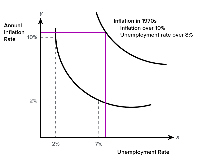
Stagflation, then, is defined as the situation where both unemployment and inflation are high, contrary to the Phillips curve. It occurs when policy actions fail to boost economic growth and the economy instead becomes stuck in this seemingly impassable position.
Source: THIS TUTORIAL WAS AUTHORED BY KATE ESKRA FOR SOPHIA LEARNING. PLEASE SEE OUR TERMS OF USE.
