Market and Firm Outcomes in Monopoly

1. Modeling the Short Run in a Monopoly Market

Let’s examine how the firm interacts with the market in the short run in a monopoly market. We will first examine the relationship of the firm to the market, and then review the profitability status of the firm in the short run, before examining the long run outcomes.

1a. The Market and the Firm

In a monopoly market a firm is known as a price setter, because the selling price will be set by the seller along its downward-sloping demand curve.

Suppose that Ride-on-Reading is a railway servicing three Midwest states. It is the only flatcar railway service available for carrying oversized and oddly-shaped freight in these states. The data in the table reflects the firm’s pricing and revenue situation. Price (column 2) is measured in thousands of dollars per the number of flatcars in service. The firm sets the price for each quantity of flatcars in service. Notice that in row one, if the firm is selling nothing, then the price of $11,000 is too high even for a monopoly.

Unlike a perfectly competitive firm, a monopoly must reduce the price in order to sell the next unit of output. You might wonder, why? It is because in a monopoly market, the firm is the market. Market demand is typically downward-sloping, and adheres to the law of demand. As price falls, buyers purchase larger quantities. This inverse relationship is shown in column 1 (Quantity) and column 2 (Price) in the table above.

hint

In a monopoly market, the firm and the market are synonymous. When there is only one seller or dominant supplier, then that firm is the market, because there are no close competitors for that product.

Because the price is no longer the same for each unit of output, total revenue will not be increasing by the same amount every single time, which also means marginal revenue will not be equal to the price. Price (column 2) is greater than marginal revenue (column 4) (P > MR), except in the first row where output is zero.

think about it

Do you think any profit-maximizing firm would produce at MR < 0? If marginal revenue is the added revenue for the next unit, and marginal revenue is negative, would that imply that selling the next unit reduces total revenue?

hint

You find marginal values by calculating the difference between two total values, then dividing by the difference in two quantities. For example, take the difference between row two and row one for the total (product, cost, revenue), and divide it by the difference between row two and one for the quantity (workers, output).

In the table notice that price, marginal revenue, and average total revenue decline as quantity of output increases. Also, note that price and average total revenue have the same numeric values at each level of output. Both decline as quantity produced increases.

We can visualize these relationships by plotting quantity output on the horizontal x-axis, and price on the vertical y-axis. At an output of one flatcar, the values for marginal revenue and average revenue are identical. The marginal revenue curve lies below the average revenue curve for all other quantities in the graph.

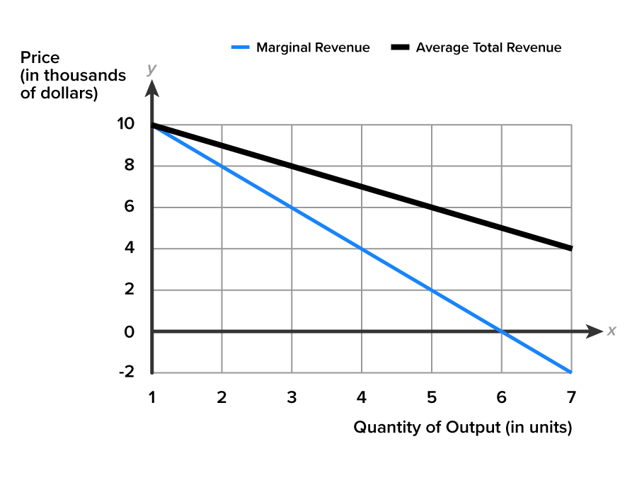
Recall that each point on the average revenue curve represents the price of the product and quantity sold in the market. A demand curve also relates the price of the product and the quantity sold in the market. Average revenue represents the firm’s product demand, and the average revenue curve represents the firm’s demand curve in the market. Since the firm is the market, the demand curve is downward-sloping.

Let’s review the cost side of the monopoly firm, Ride-on-Reading, in the table below. As expected, total cost (column 2), which represents fixed plus variable cost, rises as quantity of output increases. It costs more to produce more. While fixed cost will be unchanged, variable cost associated with variable inputs like labor and raw materials will rise as production increases. In the table, marginal cost (column 3) begins high, then drops before rising again. We expect a J-shaped curve for marginal cost. The data in the table reflects that J-shape, beginning at $5, and then dipping down to $1, before gradually rising up to $13. The data on average total cost (column 4), which begins at $9, and dips down to $4, before rising back up to $7, suggests that the ATC curve should have the typical U-shape.

In the case of a monopoly there is no market supply curve. Instead the firm is the market, and the firm’s short-run supply curve (S) replaces market supply. The short-run supply curve (S) begins on the MC curve at or above where price equals AVC, or the shutdown point, and continues upward along the MC curve.

hint

The monopolist is a profit-maximizer and sets the price.

Let’s review the revenue, cost and profit situation in the table. The firm’s profits are maximized, or loss minimized, when the distance between TR and TC is the largest. Scan down through the total profit (column 4) in the table. The largest total profit is $12 at both a quantity of three and four flatcars. By using the profit-maximizing rule of equating MR and MC, we can be more precise about the quantity of output to produce.

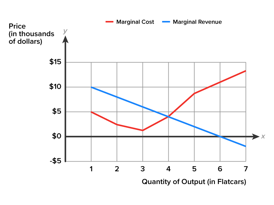
Every firm in any market, whether the firm is a price taker or a price setter, maximizes profit by choosing the level of output where MR = MC. Use the graph to determine the monopoly firm’s profit-maximizing level of output. Locate where MR and MC intersect and follow that point down to the horizontal x-axis. This occurs at the quantity of four flatcars.

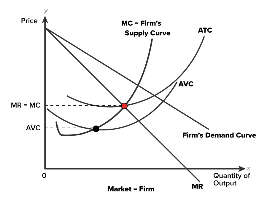
Let’s review this case of the firm as the market. Take note that in the graph below both the demand and marginal revenue curves are downward-sloping. Why? Because the firm is a price setter, and can only sell an additional unit if it lowers the price. As the price declines, the added revenue for selling an added unit also declines. The range of price elasticity along a downward-sloping demand curve will include price elastic toward the upper portion of the curve, unit elastic at a midpoint of the curve, and price inelastic in the lower portion of the curve. If the selling price is in the elastic range, then lowering the price will increase total revenue. But if the selling price falls into the inelastic range, then raising the price will increase total revenue.

The two cost curves in the graph, ATC and AVC, have the expected shapes. The average total cost curve lies above the average variable curve, and both have the typical U-shape. The marginal cost curve is J-shaped and intersects both average curves at their minimum points.

hint

• The short-run supply curve (S) begins on the MC curve at or above where price equals AVC, that is, the shutdown point, and continues upward along the MC curve. The firm is willing and able to produce and sell these quantities of output at their corresponding prices.
• Notice that in the graph above the MR is below the horizontal axis. This is because MR can be negative.

term to know

Short-Run Supply Curve

Every point along the MC curve beginning at or above price equals AVC, the shutdown point.

1b. Short-Run Profitability

If a monopoly firm is a price setter does it always earn more than normal profits?

In the short run, a price setting firm will seek the quantity of output along its downward-sloping demand curve where profits are highest or, if profits are not possible, where losses are lowest. Margins tell the firm what to do. Should production be higher or lower than it is currently? And the best any firm can do is to follow the profit-maximizing rule, equating MR = MC. Once the quantity of output has been selected, then the price is known. The firm’s total revenue, total cost, and level of profits are determined.

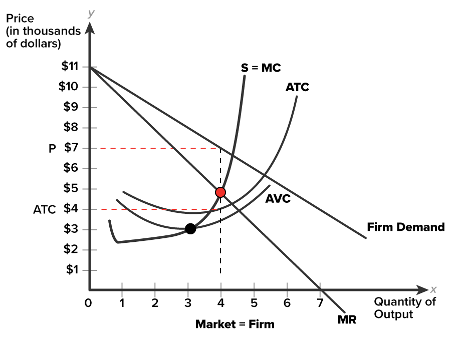
According to the graph, our monopoly firm, Ride-on-Reading, will produce the profit-maximizing output level of four flatcars. The revenue and cost tables show that at four units of output, the selling price for the service for $7,000 with ATC of $4,000 and MR of $4,000

To determine short-run profitability, the firm subtracts price per unit and average cost per unit (P - ATC), then multiplies the numeric value by the four units of output. The difference between price ($7,000) and ATC ($4) is $3,000. If you multiply $3,000 by four units the result is $12,000. The firm is–not surprisingly–earning profit!

The graph illustrates Ride-on-Reading’s current situation. The demand curve and marginal revenue curve (MR) are downward-sloping. To profit-maximize, the firm will locate where MR crosses MC. In the graph, follow the dashed line down from where MR = MC to the horizontal quantity of output axis. The profit-maximizing quantity of output for the firm is four units. Next, follow the dashed line up to the demand curve, then across back over to the vertical price axis. Selling price is $7,000.

Averages tell the firm how well it is doing. In the graph above, the ATC curve lies below the demand and marginal revenue curves. Locate ATC along the dashed line for MR = MC. Trace that ATC point across to the vertical axis at $4,000. In the graph, notice the rectangular area formed by the dashed lines between price $7,000 and ATC $4,000 and between zero and four on the horizontal axis. This area is referred to as the profit box.

To calculate the area of the profit box–the rectangle between Price and ATC and quantity of 4–we can use the formula: base * height. If we calculate the area of this rectangle, we will know the value of short-run positive economic profits, which are profits that exceed normal profits.

formula to know

Area of Rectangle

The base is 4 - 0 = 4 units, and the height is $7,000 - 4,000 = $3,000. If you multiply four units times $3,000, the result is $12,000. This monopolist is making positive economic profits, which are profits that exceed normal profit. Is this outcome what you would expect from a monopolist?

1c. Short-Run Disturbance

Does a monopolist always earn profit in excess of normal profit? Since a monopolist sets the product price, it would seem a logical conclusion that profits always exist.

However, we must account for changes in the non-price factors of demand and supply that are disturbances to a market in equilibrium. If a non-price factor of demand changes and causes the curve to shift, then the product price will adjust upward or downward in response. This will affect a firm’s short-run profitability.

Let’s analyze another set of graphs to see if a monopolist earns profit in excess of normal profit if average total costs rise.

hint

For a monopoly firm, the profit-maximizing condition is MR = MC. With a downward-sloping demand curve this means P > MR and P > MC.

In the graph, the profit-maximizing level of output is four units at a selling price of $7 per unit. Locate where MR and MC cross. Next, follow the vertical dashed line down from where MR crosses MC to the horizontal axis of quantity of output. We can confirm four units. Now follow the same dashed line to the demand curve, and across to the vertical price axis at $7. We have confirmed the selling price. Notice that price located at $7 is higher than where MR and MC are equal at $5, thus, price is greater than marginal cost (P > MC).

key concept

Price > ATC Firm earns economic profit.
Price = ATC Firm earns normal, or zero economic profit.
Price < ATC Firm earns an economic loss.
Price < AVC Firm shuts down temporarily.

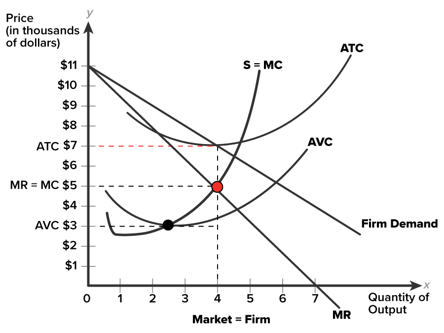
Averages tell the firm how well it is doing. In the graph, locate ATC along the vertical dashed line for MR = MC by following it up to the ATC curve. ATC lies tangent to the demand curve for the quantity of 4 units. Trace the ATC point across to the vertical price axis at $7,000. If price per unit is $7, and average per unit cost is $7, the difference between P - ATC is zero. This suggests the monopolist is earning zero economic profits, rather than positive economic profits. The firm is earning normal profit and receiving a fair return on investment, an implicit cost.

If the firm is just breaking even, should the firm continue to produce? The decision to continue or shut down temporarily is dependent upon whether the firm is covering its average variable costs, which includes payment to the labor input. The firm should not shut down if breaking even.

Check the graph above again. This time look for the AVC curve. Follow the vertical MR = MC dashed line down to its intersection with the AVC curve. Price ($7,000) is greater than AVC ($3,000), so P > AVC. The firm is able to cover its variable costs and some of its fixed costs. It should continue to produce. A firm will shut down temporarily when P < AVC.

Suppose instead of breaking even, the firm’s situation is illustrated by the graph below. Is the firm making short-run profits? Should the firm continue to operate or shut down temporarily?

try it

Use the graph to identify the firm’s profit-maximizing level of output and price where MR = MC. What is profit maximizing level of output and selling price?

Quantity of output is 4 units; selling price is $7,000.

Determine the firm’s short run profit situation. Use the graph to identify the ATC for four units of output. What is the relationship between selling price and ATC?

Selling price is $7,000 and ATC is $8,000. P < ATC. The firm is loss minimizing.

Determine if the firm should continue to operate or shut down temporarily. Use the graph to identify the AVC for 4 units of output. What is the relationship between selling price and AVC?

Selling price is $7,000 and AVC is $3,000. P > AVC. The firm should continue to operate.

big idea

A firm producing where price equals average variable cost (P = AVC) is only able to cover its variable costs through its sales. This is the shutdown decision point.

• When a firm can cover its average variable cost (P > AVC), then the firm will operate at a loss. Sales revenue will cover the variable cost but not all fixed costs. By continuing to operate, losses will be minimized but not eliminated.
• When a firm cannot at least cover its average variable cost (P < AVC), it should consider shutting down temporarily until market conditions improve.

2. Modeling the Long Run in a Monopoly Market

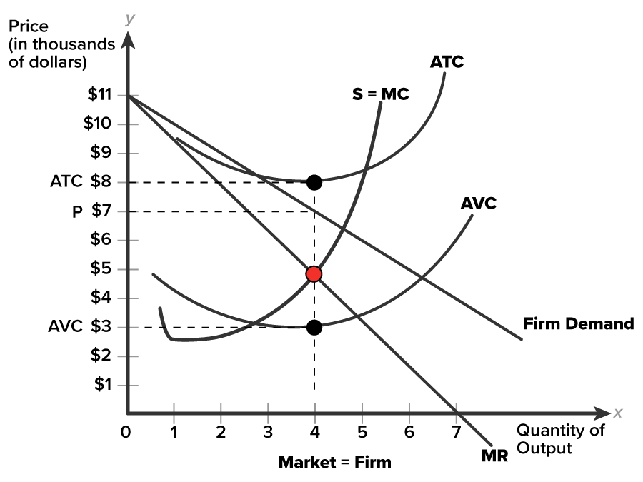
Will profits persist for a monopolist? In the case of a monopoly, positive economic profits will not attract new investment from sources outside the monopoly market, because barriers prevent new firms from entering the market. In long-run equilibrium positive economic profits may persist. Historically, exceptional profits have often inspired innovation that undercuts a monopolist’s good or service.

EXAMPLE

The U.S. Postal Service used to be the sole carrier of mail, which included both first-class letters and packages. The use of email, texting, and video calls have affected the volume of postal mail. Packages are now carried by a number of other service providers as well, including FedEx, UPS, and DHL, so the USPS has lost its monopoly on package carrying.

When we consider economic losses we must differentiate between a private and a public monopoly. If a privately-owned monopoly suffers sufficient losses in the short run, then it will exit the market when fixed costs become variable. A public monopoly established by government legislation will likely receive funding support to help offset economic losses. The U.S. Postal System has experienced significant financial losses, but still operates through taxpayer support.

Monopolies are less efficient than perfectly competitive firms. Perfectly competitive firms operate at the minimum point of their ATC curve where the MC curve intersects if from the bottom. This indicates that the firm’s production is at capacity, or the maximum possible output given its available resources.

A monopolist has the ability to operate at the capacity output, producing a larger possible output given its available resources, but chooses to under-utilize its capacity. This is known as having excess capacity. Because monopolists do not produce at the minimum of the ATC curve, the firm is productively inefficient. The monopolist chooses to restrict output to maintain a higher price.

All firms profit-maximize at MR = MC. The selling price for a perfectly competitive firm is equal to marginal cost (P = MC). And buyers purchase the product at the lowest possible price. Perfectly competitive firms produce at an output level where the price (P) equals the marginal cost (MC) of production. This is known as allocative efficiency.

For a monopoly firm a downward-sloping demand curve means P > MR and P > MC. Because monopolists charge a selling price above marginal cost (P > MC), Monopolists are allocatively inefficient. Buyers will suffer because price (P) is a measure of how much buyers value the good, and the marginal cost (MC) is a measure of what an extra unit cost society to produce. If P > MC, then the marginal benefit to society (as measured by P) is greater than the marginal cost to society of producing additional units, and a greater quantity should be produced.

key concept

For a monopoly firm, the profit-maximizing condition is MR=MC. With a downward-sloping demand curve this means P > MR and P > MC.

Monopolists are not productively efficient, because they do not produce at the minimum of the average cost curve. Monopolists are not allocatively efficient, because they do not produce at the quantity where P = MC.

As a result, monopolists produce less and charge a higher price then a combination of firms would in a perfectly competitive industry. Monopolists also may lack incentives for innovation, because they need not fear the entry of new competitors.

watch

This video reviews the monopoly model, graphically.

terms to know

Excess Capacity

The firm is producing a quantity of output that under-utilizes its potential capacity.

Allocative Efficiency

Producing at an output level where the price (P) equals the marginal cost (MC) of production.

Productive Efficiency

Producing goods and services for the lowest cost, the minimum of ATC.