Table of Contents |
As you may recall from previous coursework, the slope of a line between two points is  which is often represented as
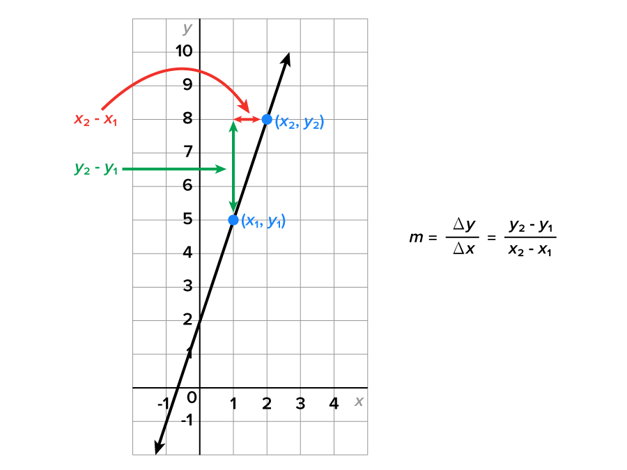
Consider the graph shown. Given two points on a line, which we call  and
and  we calculate the slope as follows.
and  is given by
 the slope can also be written
EXAMPLE
Consider the points and
and 
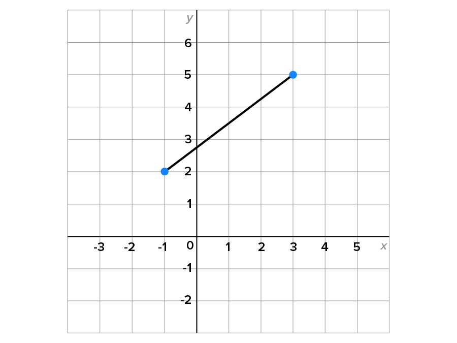
 and
and  then use the slope formula.

EXAMPLE
Consider the points and
and 
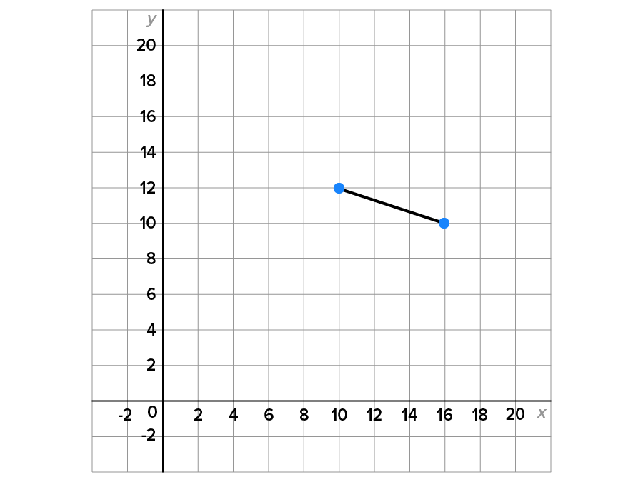
 and
and  then use the slope formula.
 to
to  move down 2 units, then to the right 6 units. This translates to
EXAMPLE
Consider the points and
and 
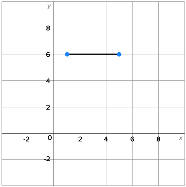
 and
and  then use the slope formula.

Note that the lines in all three examples were functions. Based on this simple fact, we define a linear function as a function whose graph is a line.
Here is a problem for you to try.
 and
and 
 the slope is:

When x and y represent quantities, the slope can be interpreted as a rate of change.
EXAMPLE
Suppose that in 2017, the population of a small town was 4,124 and in 2021, the population rose to 5,000.
 the population of the town and
  the year, then we have two ordered pairs to describe the situation:
  and
and 


Here is a problem for you to try on your own.
 minutes.
 miles.


Now that we have made the connection between slope and linear functions, let’s take a closer look at how these ideas intertwine.
There are four forms that are used to represent a function: word form, equation (function) form, table form, and graph form. Through this tutorial, we will see how these are connected when the situation is modeled by a linear function.
A key connection to make is between the equation of the linear function, its corresponding table of values, and its graph.
Consider the equation 
Here is a table of values:

|
0 | 1 | 2 | 3 | 4 |
|---|---|---|---|---|---|

|
3 | 5 | 7 | 9 | 11 |
Here is the graph of this function:
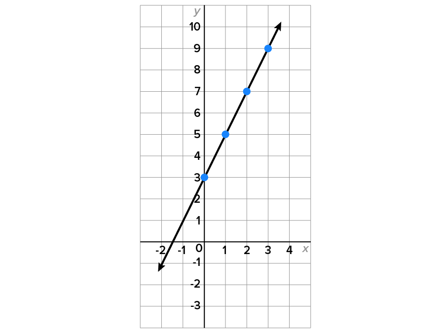
Note that  is a linear function, and therefore must have a slope.
Let’s take two input-output pairs:  and
and 
Calculate the slope between them: 
Let’s choose two other points:  and
and 
Calculate the slope between them: 
In fact, given that the graph is a line, the slope of the line between any two points should be 2.
Notice also that when 
 This means that the graph has y-intercept
Given the equation of any linear function,  we can make some generalizations.
 or using function notation,
 is on the line.
You may remember from previous coursework that the equation has a special name, called the slope-intercept form.
The slope-intercept form of a line is the most convenient to use to model situations. Through the next few examples, we will see how the graph, table, function, and verbal descriptions relate to each other.
EXAMPLE
John is mountain climbing and begins his journey at an elevation of 500 feet. He also ascends at a rate of 80 feet per hour. the number of hours that John is ascending, and
  his elevation after t hours. Since John is ascending at a constant rate, a linear function can be used to model this situation.
 hours hours
|
0 | 1 | 2 | 3 | 4 | 5 |
|---|---|---|---|---|---|---|
 elevation (feet) elevation (feet)
|
500 | 580 | 660 | 740 | 820 | 900 |
 increases by 80 units for every unit that t increases.
 Since t is the input and is the output, our model will have the form
 is 500 feet, indicating that this is the y-intercept. From the table above, the constant rate of change is 80 feet per hour, indicating that the slope of the model is 80.
 is an increasing function.
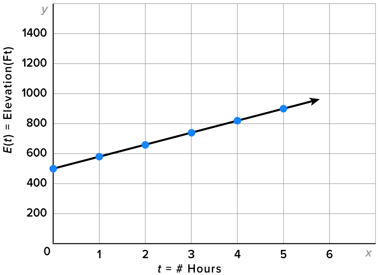
 Even though the expression for is defined for all possible values of t, only nonnegative values of t will provide meaningful results. This is because John can’t climb mountains for a negative amount of time.
Now that we have this insight, writing the equation of a linear function will be a bit easier.
EXAMPLE
A basement has flooded. After pumping begins, the amount of water (in gallons) in the basement t hours after pumping began is given by the function

|
hours
|
0 | 1 | 2 | 3 | 4 | 5 |
|---|---|---|---|---|---|---|
 gallons remaining gallons remaining
|
8000 | 6800 | 5600 | 4400 | 3200 | 2000 |
 decreases by 1200 units.
is decreasing.
decreases by 1200 units.
is decreasing.
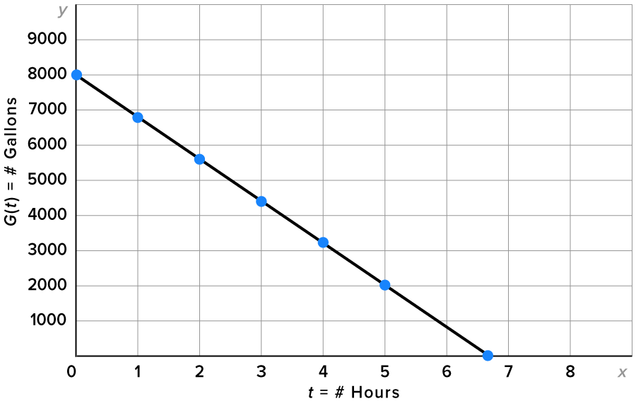

|
Set to 0.
|

|
Replace with 
|

|
Subtract 8000 from both sides. |

|
Divide both sides by -1200. |

|
Simplify. |
 hours. Or 6 hours and 40 minutes. This is represented on the graph by the t-intercept.
We have seen examples with rates of change that led to increasing and decreasing functions. Now, let’s look at one where the function is constant.
EXAMPLE
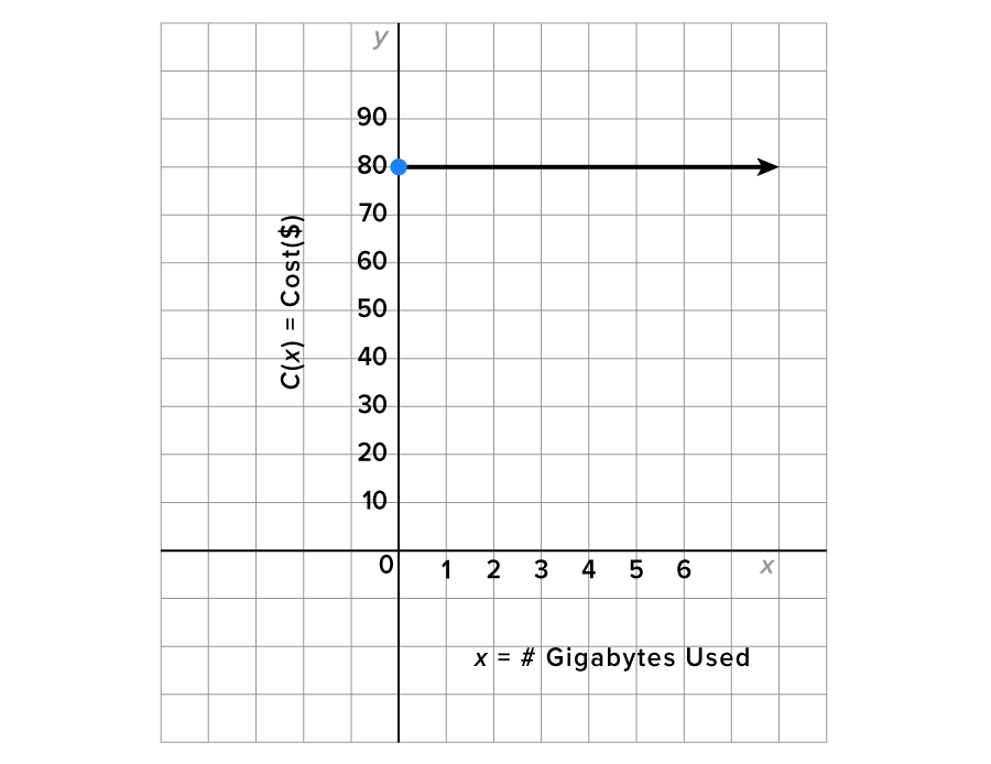
A cellular phone plan costs $80 regardless of how much data is used. Let the cost of the plan after using x gigabytes of data.
|
|
0 | 1 | 2 | 3 | 6 | 20 |
|---|---|---|---|---|---|---|

|
80 | 80 | 80 | 80 | 80 | 80 |
 Regardless of the input, the output is 80, which represents a plan cost of $80.
 is a constant function.
The equation in the last example was written To align with the slope-intercept form, it could also be written  This means that the slope of the line is 0. Through the last three examples, this leads to an important connection between the slope of the line and whether its corresponding function is increasing, decreasing, or constant.

 indicates that
  is increasing.
 indicates that is decreasing.
  indicates that is constant.
Here is an example that is very applicable to everyday life: converting between Celsius and Fahrenheit.
 where m is the slope (constant rate of change) and is the y-intercept.
SOURCE: THIS TUTORIAL HAS BEEN ADAPTED FROM OPENSTAX "PRECALCULUS” BY JAY ABRAMSON. ACCESS FOR FREE AT OPENSTAX.ORG/DETAILS/BOOKS/PRECALCULUS-2E. LICENSE: CREATIVE COMMONS ATTRIBUTION 4.0 INTERNATIONAL.
A function whose graph is a line.
A linear equation in the form  where m is the slope (constant rate of change) and
  is the y-intercept.
The slope of a line containing the points  and
and  is given by
Using function notation, where  the slope can also be written

