Use Sophia to knock out your gen-ed requirements quickly and affordably. Learn more
×

Inventory Management Techniques

Author: Sophia

what's covered
In this tutorial, we will address the techniques to measure and calculate the costs of inventory. In particular, this tutorial will cover:

Table of Contents

1. The Economic Order Quantity Formula

You may recall from earlier in this challenge that the main goal of inventory management is determining the optimal amount of inventory to keep for both salable goods and the raw materials to make them. There are several strategies for calculating these levels.

One of the oldest is economic order quantity (EOQ), a process for determining the optimal amount of an item to order at one time to minimize holding costs (also referred to as carrying costs), the amount it costs to keep a unit in inventory, including storage, depreciation (loss of value over time), and shrinkage (theft, damage, etc.). Effective inventory control is paramount for optimizing profitability. Holding costs, the expenses associated with storing unsold inventory, can significantly impact a company's bottom line. These costs encompass storage space, labor for managing inventory, insurance, taxes, and potential obsolescence or spoilage of goods.

hint
You can use this spreadsheet to see the examples and test the formulas without having to pull out a calculator. You may also use it to solve the problems below.
Inventory Optimization.xlsx

Holding costs are determined by multiplying the cost of an item by a known percentage, usually about 20% for nonperishable goods, which itself is determined by dividing total inventory costs by total value of inventory. Some of the specific components of holding costs include the cost of storage, such as the cost of rent for a warehouse, insurance on the goods stored in the warehouse, inventory handling costs, such as the maintenance of forklifts to move inventory, depreciation costs, such as the costs associated with obsolescence or spoilage, and the cost of the capital, which is the interest on funds used to finance the inventory (if applicable).
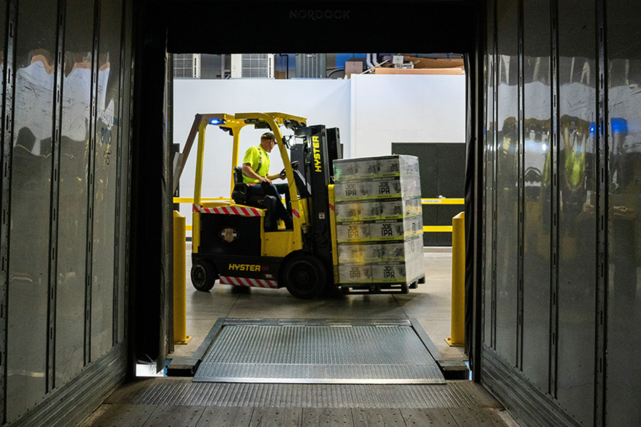
A forklift moving crates in a warehouse
Maintaining equipment used to manage inventory has costs. A forklift, for example, requires fluid replacements, hydraulic system inspections, exhaust system checks, along with many other requirements to meet safety standards. These expenses (including the time it takes to do these things) are all part of holding costs.

EXAMPLE

A bicycle store determines that the value of inventory over a year divided by inventory costs is 20%. A bicycle that costs $600 would have a holding cost of $120 ($600*20%).

Determining the EOQ, like any inventory management technique, requires good data. The values the manager needs to know, and the variables we will assign to them, are:


  • D = Demand for the product (number of units sold in a year, or used in a year for raw materials)
  • S = Setup cost per order (this includes factors like shipping and any labor costs for unpacking and storing the items)
  • H = Holding cost, as explained above, which is reached by multiplying the cost of an item by a percentage, usually about 20%
From these three values, the formula for determining EOQ is:

E O Q equals square root of fraction numerator 2 D times S over denominator H end fraction end root

try it
Let’s say that Gordon’s favorite bike shop sells 12 of his bikes in the first year for $600 each. Their holding cost is 20%, so the cost for storing Gordon’s bicycles is $120 per bicycle. Their setup cost is $20 per order, for the labor of assembling the bicycle for the showroom floor.
What is the EOQ for the bike shop? That is, how many bikes should they order for the coming year?
We know that D (demand) is 12, S (setup cost) is $20, and H (holding cost) is $120 per bicycle. We can plug these numbers into the equation to determine EOQ, the ideal inventory quantity we are trying to reach.

E O Q space equals square root of fraction numerator 2 times 12 times 20 over denominator 120 end fraction end root

E O Q space equals square root of 480 over 120 end root

E O Q space equals square root of 4

E O Q space equals 2
The bicycle shop should order two of Gordon’s bicycles at a time. If we had arrived at a decimal, we could round the number for an optimal number. Moreover, for high-quantity items, the inventory manager must round to the order quantity (the number of items that must be ordered at a time).

While EOQ is relatively easy to find using a calculator, it has some limitations. Underlying assumptions are:

  • The ordering cost is constant.
  • The rate of demand is known and spread evenly throughout the year.
  • The lead time is fixed.
  • The purchase price of the item is constant (i.e., no discount is available).
  • The replenishment is made instantaneously; the whole batch is delivered at once.
  • Only one product is involved for each calculation.
As you might guess, none of these assumptions are safe. For example, suppose holding rent or insurance increases—this would then impact the holding rate, which would impact the outcome. However, the EOQ gives a relatively good estimate for most inventory purposes, and because these calculations can be entered in a spreadsheet, it can be applied to a long list of items all at once.

terms to know
Economic Order Quantity
The optimal quantity of an item to order at a time; also refers to the formula for calculating this number.
Holding Cost
The cost of keeping an item, including storage, insurance, depreciation, etc. It is often calculated as 20% of the item’s cost.


2. The Total Cost Formula

The EOQ formula considers an optimal order quantity for a single product. However, there are a number of other questions an inventory manager might have, such as how often to place orders. Another formula they can use is the total cost formula to determine annual inventory costs. The total cost formula determines the total cost for ordering items. An inventory manager can change variables within the formula to see how changes in practice will affect the total cost.

Recall the three values we used to determine EOQ (the optimal quantity to keep in inventory):

  • D = Demand for the product (number of units sold in a year, or used in a year for raw materials)
  • S = Setup cost per order (this includes factors like shipping and any labor costs for unpacking and storing the items)
  • H = Holding cost, as explained above, which is reached by multiplying the cost of an item by a percentage, usually about 20%
To this list we can add two more data points:

  • Q = The quantity of an item that is ordered at a time. This will be the same as EOQ if this is already determined; otherwise, it may be the minimum number that can be ordered at once.
  • C = The wholesale cost per item (the order cost divided by the quantity received; note that this is the cost to the store or company, not the final price for customers).
The total cost formula is shown below. Remember that all of these are usually for one year.

Total space Cost space left parenthesis TC right parenthesis space equals space Purchasing space Cost space left parenthesis PC right parenthesis space plus space Ordering space Cost space left parenthesis OC right parenthesis space plus space Holding space Costs space left parenthesis HC right parenthesis

However, each of these items must be calculated first.

  • The purchasing cost (PC) is the cost per item (C) times the demand (D).
  • The ordering cost (OC) is the demand (D) times setup cost (S), divided by the number of items per order (Q).
  • Holding cost, remember, refers to the cost for maintaining inventory and is often calculated as a percentage of the cost. In this formula, the holding cost (HC) is the per unit holding cost (H) times the quantity per order (Q), divided by two. The reasoning behind the final step is that as items are sold and restocked, inventory is, on average, half-full.
With this understanding, we can now write out the full formula:

T C space equals C times D space plus fraction numerator D times S over denominator Q end fraction plus fraction numerator H times Q over denominator 2 end fraction

IN CONTEXT

Let’s return to the bicycle shop and consider a product sold in higher quantity, bicycle locks. The store sells 750 locks a year. The locks are ordered in batches of 40 for $4 per item, have a modest setup fee of $10 per order, and a holding cost of $1 per lock (15% of the retail cost). The shop has already determined the EOQ is 120 (rounded down to a factor of 40, since they are sold in packs of 40).

To determine the total holding cost, let's plug the numbers into the formula.

T C equals C times D   plus   fraction numerator D times S over denominator Q end fraction plus fraction numerator H times Q over denominator 2 end fraction

T C equals 4 times 750   plus fraction numerator 750 times 10 over denominator 120 end fraction   plus fraction numerator 1 times 120 over denominator 2 end fraction

We can calculate the total cost for this item at $3,000 (the purchasing cost, 750*4) plus $62.50 (the ordering cost, 750*10/120), plus $60 (the holding cost, 1 x 120/2). The total cost is thus $3,122.50.

The formula can be used to help determine how changes in practice would impact the total cost. For example, the bicycle store might wonder if they should order 240 locks at a time instead of 120. The cost per lock is slightly cheaper with larger orders, at $3.90 per unit instead of $4.00. This change would double the setup costs, since it takes twice as long to ship, unpack, price, and shelve twice as many locks. The holding costs also go up since the locks are taking up more space, and the store must drop another item to make room. These are called opportunity costs, the loss of potential gain from alternative use of resources. For these reasons, the holding cost will be $1.50 per lock instead of $1.00.

How would doubling the quantity ordered affect total cost? We can insert the new numbers into the formula to find out.

T C equals C times D   plus   fraction numerator D times S over denominator Q end fraction plus fraction numerator H times Q over denominator 2 end fraction

T C equals 3.90 times 750   plus fraction numerator 750 times 20 over denominator 240 end fraction plus fraction numerator 1.50 times 24 over denominator 2 end fraction

The purchasing cost at the expanded order size will be $2,925. Although the quantity per order is increased and the setup cost per order has increased, these are offset by fewer orders, so the order cost is the same. Finally, the holding costs are increased due to opportunity costs.

T C equals 2925   plus   62.50 plus 180 space

The total cost now adds up to $3,167.50, which is more than their current total cost, despite the discount for a larger order. This is due to opportunity cost—that is, the larger orders would mean dropping another product to make room on the shelf for more locks.

terms to know
Purchasing Cost (PC)
The total annual cost for an item, calculated by multiplying the cost per unit by demand.
Ordering Cost (OC)
The cost per order, calculated by dividing the purchasing cost by the quantity per order.
Opportunity Costs
The loss of potential gain from alternative use of resources, such as store space that could be used to sell other goods.


3. ABC Technique

The examples above are for nonperishable goods, but for many situations across the supply chain, there are some materials or products that require special handling, special storage, or which must be used immediately. Materials management is a field within operations management that specializes in procurement and storage of a variety of materials, some that require special handling.

ABC analysis is an inventory categorization technique often used in material management. It is also known as “selective inventory control.” The essence of ABC analysis is to assign grades to materials based on the need for control and recordkeeping.

  • A items: Very tight control and accurate records
  • B items: Less tightly controlled and sufficient records
  • C items: Simplest controls possible and minimal records
The ABC analysis provides a mechanism for identifying items that will have a significant impact on overall inventory cost and production goals, while also providing a mechanism for identifying different categories of stock that will require different management and controls.

EXAMPLE

A restaurant will have some items that are high cost, require refrigeration, and must be used immediately, such as meat and seafood. These A items are also the most crucial to the menu and daily operations of the restaurant. B items, like onions and potatoes, would have a longer shelf life and may not require refrigeration, but still must be used within a certain timeframe. C items would have a very long shelf life, such as dry grains, salts, and oils.

A items are very important for a business. Because of the high value of these A items, frequent value analysis is required. In addition to that, a business needs to choose an appropriate order pattern (e.g., “just-in-time”) to avoid excess capacity.

B items are important, but less important than A items; they may require modest analysis but will not have as much impact on total costs.

C items are least important, at least in terms of inventory management. They tend to be less expensive items that have a long life and can be stored in large quantities.

The use of an ABC analysis can help set different holding costs for items that are more expensive, cost more to store, and have more risk (such as meat and seafood going bad). ABC analysis is also crucial to purchasing schedules. A store without an ABC inventory model is likely to have uniform purchasing, where all materials are ordered on the same schedule, such as once a month. A store using an ABC model is likely to have weighed purchasing, where each category has its own schedule.

EXAMPLE

A restaurant might make A purchases (meat, seafood, dairy, etc.) every 2–3 days, B purchases (fruits, vegetables, etc.) once a week, and C purchases (dry goods, oils, etc.) once a month. As you’ve guessed, making a “mistake” and over-ordering or under-ordering C purchases does not have much impact, while making a mistake on A purchases could mean the restaurant runs out of critical menu items!

terms to know
Materials Management
A field within operations management that specializes in procurement and storage of a variety of materials, some of which require special handling.
ABC Analysis
An inventory categorization technique often used in material management that assigns grades to materials based on their need for control.


4. Just-in-Time Systems

As we learned earlier, just-in-time (JIT) is a production strategy striving to optimize costs by reducing in-process inventory and associated holding costs. While the JIT process might seem to be the simple practice of operating without (much) inventory, it still relies on inventory management of the resources used to make their goods. For the materials manager, this is quite different from a more traditional inventory method.

  • Supply is synchronized with production demand, and the optimal amount of materials are on hand at any time. Supplies may come in at intervals throughout the production day instead of once a week or once month, when parts move directly from the truck to the point of assembly, with little or no need for storage.
  • The materials manager must be in constant contact with suppliers to specify needs. A company without inventory relies heavily on suppliers being responsive, reliable, and punctual. This makes supplier relationships extremely important.
  • There is even less margin for error in the supply chain. The materials manager must be aware of any potential shortages that will impede workflow.
  • Labor for setup fees is reduced since materials are sent directly to production; there is no time needed to store, then retrieve, materials in a warehouse or storage room.
  • There is a smaller chance of inventory loss through theft, breakage, or other causes.
  • There may be times with no production underway (such as changing over to a different production item or method) where there is no inventory.

EXAMPLE

If Gordon decides on a JIT system for his bicycle company, he will need less space and lower costs, but he will need to be in constant contact with suppliers and runs the risk of production halting if any component is not delivered promptly.

In terms of day-to-day work, the inventory manager for a JIT manufacturer will be on the floor most of the day, receiving and directing supplies. They will likely be on the phone calling suppliers throughout the day. A more traditional manager would do more long-term planning from their office, determining holding costs, scouting out suppliers, and perhaps overseeing occasional shipments at the warehouse.

To achieve continuous improvement, it is crucial to have good communication between the materials manager and the workers they support. For example, a shop may use a Kanban system; taken from the Japanese word for signboard, a Kanban system is any highly visual project management tool that communicates where a product is in the production cycle, as well as any needs that must be filled by the materials manager. This may be as simple as a highly organized shelving system so the materials manager can see what materials are low in stock, but it may be a digital system where materials are scanned, and the materials manager can receive an alert when a material falls below a certain level. Whatever the system, it is crucial for clear and reliable communication from employees, whether it is remembering to scan materials so inventory measures are accurate or some other visual queue, even a brightly colored sticky note on the shelf that needs refilling.

two office workers arranging post it notes in columbs
A Kanban system can be used to organize projects and processes. Sometimes, Kanban systems are as simple as the use of sticky notes.

Implemented correctly, JIT focuses on continuous improvement and can improve a manufacturing organization’s return on investment, quality, and efficiency. There are other advantages and disadvantages to a just-in-time system not directly related to inventory or materials management.

term to know
Kanban System
A highly visual project management tool that communicates where a product is in the production cycle, as well as any needs that must be filled by the materials manager.

summary
We explored various inventory management strategies, including the economic order quantity (EOQ) formula, which is used to determine the optimal quantity of an item to order at one time, and the total cost formula, which shows annual holding costs for an item and can be used to determine how process changes will affect the total cost. ABC analysis is one form of selective inventory control, when some items have a shorter shelf life or need special handling. Finally, there are just-in-time (JIT) systems, which involve largely operating without inventory and thus require operations managers to be active in coordinating delivery of materials. The best method for inventory management will largely depend on the nature of the company.

Source: This tutorial has been adapted from Saylor Academy and NSCC “Operations Management”. Access for free at https://pressbooks.nscc.ca/operationsmanagement2/. License: Creative Commons Attribution 4.0 International.


Terms to Know
ABC Analysis

An inventory categorization technique often used in material management that assigns grades to materials based on their need for control.

Economic Order Quantity

The optimal quantity of an item to order at a time; also refers to the formula for calculating this number.

Holding Cost

The cost of keeping an item, including storage, insurance, depreciation, etc. It is often calculated as 20% of the item’s cost.

Kanban System

A highly visual project management tool that communicates where a product is in the production cycle, as well as any needs that must be filled by the materials manager.

Materials Management

A field within operations management that specializes in procurement and storage of a variety of materials, some of which require special handling.

Opportunity Costs

The loss of potential gain from alternative use of resources, such as store space that could be used to sell other goods.

Ordering Cost (OC)

The cost per order, calculated by dividing the purchasing cost by the quantity per order.

Purchasing Cost (PC)

The total annual cost for an item, calculated by multiplying the cost per unit by demand.