In this lesson, you will learn how to identify characteristics of time series data. Specifically, this lesson will cover:
1. Introduction to Time Series and Forecasting
Time series analysis is a method used to analyze data points collected or recorded at specific time intervals. This type of data is called a time series. Examples include daily stock prices, monthly sales figures, or yearly rainfall totals.
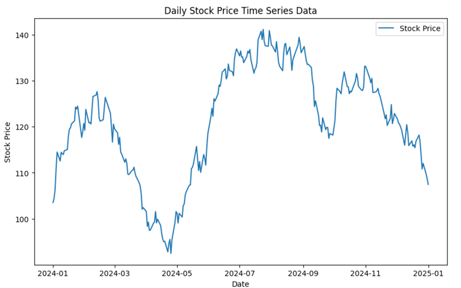
The line chart below shows what time series data looks like. The x-axis represents the dates, and the y-axis represents the stock prices. The data points show slight fluctuations from day to day, which is typical for stock prices. In general, when you visualize time series data, the x-axis will represent a date such as a day, month, or year. The y-axis will represent the value of the variable you are measuring, such as stock prices, sales figures, or temperature readings.
The main goal of analyzing a time series is to understand the underlying structure of the data and to identify any patterns. By analyzing these patterns, businesses can make better decisions, such as predicting future sales, planning inventory, setting marketing strategies, and creating accurate forecasts. Forecasting involves using historical time series data and statistical methods to make educated predictions about future events. This allows businesses to anticipate future trends and prepare accordingly, improving their ability to adapt and succeed in a dynamic market.
Before you can apply a forecasting method to time series data, you must understand and identify the essential types of patterns that can be present in time series data. Several types of patterns that you want to identify in time series data are:
-
Trends: A trend pattern is the general direction in which data is moving over a long period. It can be upward, downward, or flat.
-
Seasonality: Regular patterns that repeat at specific intervals, such as monthly or yearly.
-
Stationarity: Time series with statistical properties, like mean and variance, that do not change over time.
-
Noise: Random fluctuations in the data that do not follow any pattern. It is the irregular or unpredictable component of a time series that can obscure the underlying trends and patterns.
-
You may have heard the term “predictive modeling” before and be wondering why this tutorial is using the term “forecasting.” The term "forecasting" is specifically used with time series data because it involves predicting future values based on historical data collected at regular time intervals. Forecasting focuses on identifying patterns such as trends, seasonality, and cycles within the time series data to make educated predictions about future events.
On the other hand, "predictive modeling" is a broader term that encompasses various techniques used to predict outcomes based on historical data, not limited to time series data.
-
- Time Series
- A sequence of data points collected or recorded at specific time intervals.
- Forecasting
- Process of predicting future values in a time series.
- Trends
- The overall direction in which data points are moving over an extended period of time.
- Seasonality
- Recurring patterns that occur at regular intervals, such as every month or year.
- Stationarity
- A characteristic of a time series where its statistical properties remain constant over time.
- Noise
- Random variations in data that do not follow any discernible pattern and can hide other patterns.
1a. Identifying Trends in Time Series Data
A trend is the general direction in which data is moving over a long period. Identifying trends in time series data helps businesses make informed decisions, such as predicting future sales or planning inventory.
Types of Trends:
-
Upward Trend: When the data shows a general increase over time.
-
Downward Trend: When the data shows a general decrease over time.
-
Flat Trend: When the data remains relatively constant over time.
Below are three line graphs that illustrate these trends using the stock price data. The graph to the left shows an upward trend that the stock prices are generally increasing over time. The middle graph shows a downward trend that the stock prices are generally decreasing over time. The graph to the right shows that the stock prices remain relatively constant over time.
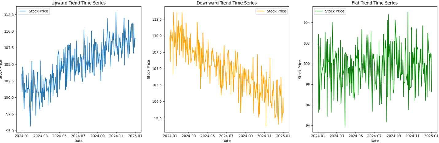
By identifying and understanding these trends, businesses can make better decisions and plan for the future. Recognizing whether data is trending upward, downward, or staying flat is a crucial step in time series analysis.
1b. Identifying Seasonality in Time Series Data
Seasonality refers to regular patterns that repeat at specific intervals over time. These patterns can be influenced by various factors, such as holidays, weather changes, or business cycles. Identifying seasonality in time series data helps businesses plan for these regular fluctuations.
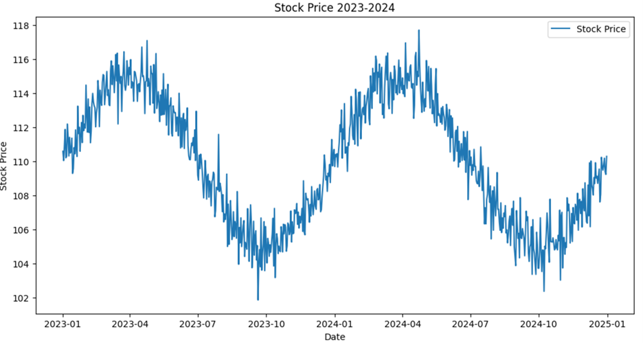
The graph below shows stock price data for two years, exhibiting a clear seasonal pattern. The stock prices reach their highest points around April each year. The stock prices dip to their lowest points around October each year. These peaks and troughs occur at regular intervals, illustrating the concept of seasonality.
The observed highs in April and lows in October in the stock price data can be attributed to seasonal factors that commonly affect many businesses and industries. For example:
Highs in April
End of Fiscal Year and Earnings Reports:
- Many companies end their fiscal year in March and report their annual earnings in April. Positive earnings reports can boost investor confidence, leading to higher stock prices.
Tax Season:
- In the United States, tax returns are due in April. Some investors may receive tax refunds and choose to invest this money in the stock market, driving up prices.
Spring Optimism:
- Spring often brings a sense of renewal and optimism. This can translate into more positive market sentiment and increased investment activity.
Lows in October
Market Corrections:
- Historically, October has seen significant market corrections and crashes (for example, the 1929 and 1987 stock market crashes). This historical context can lead to increased caution and selling pressure in October.
End of Summer and Pre-Holiday Adjustments:
- After the summer, investors might reassess their portfolios and make adjustments before the end of the year. This can lead to selling and lower stock prices.
Earnings Season Volatility:
- October is also a major earnings season. Companies report their third-quarter earnings and any negative surprises can lead to increased volatility and lower stock prices.
Seasonal patterns are essential for building accurate predictive models. By incorporating seasonality, if present in the data, you can improve the accuracy of forecasts and better anticipate market movements, in the example of the stock price data.
1c. Identifying Stationarity in Time Series Data
Stationarity is a fundamental concept in time series analysis. A time series is considered stationary if its statistical properties, such as mean and variance, remain constant over time. This consistency makes stationary time series easier to model and predict.
The key characteristics of a stationary time series are:
-
Constant Mean: The average value of the series does not change over time.
-
Constant Variance: The variability around the mean remains stable over time.
The graph below illustrates a stationary time series of stock prices over the duration of one year. The stock prices fluctuate around a mean value of approximately $50 throughout the year. This indicates that there are no long-term trends or shifts in the average price. The variance of the stock prices is $0.83, meaning the degree of fluctuation around the mean is relatively stable over time. The stock prices exhibit random fluctuations around the mean, due to the noise component. These fluctuations are small and consistent, reflecting the stationary nature of the data.
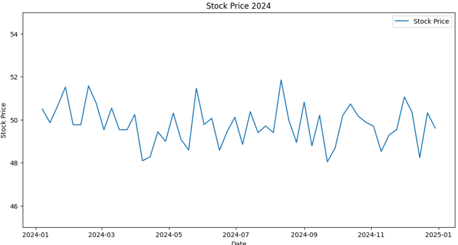
Visual inspection is a crucial first step in identifying stationarity in time series data. By plotting the data and observing its behavior over time, you can get an initial sense of whether the mean and variance remain constant. For example, in the stock price data for 2024, you observed that the prices fluctuate around a constant mean with stable variance, indicating stationarity.
However, visual inspection alone is not sufficient. Formal statistical tests are necessary to rigorously confirm stationarity. These tests provide quantitative evidence and help avoid subjective biases that might arise from visual inspection.
These tests are beyond the scope of this introductory tutorial, but they are essential tools for anyone working with time series data in a more advanced setting. They provide a more robust and reliable assessment of stationarity, ensuring that the assumptions required for many time series models are met.
By understanding and identifying stationarity in time series data, you can better apply appropriate models and make more accurate predictions in business data analytics. This knowledge is essential for analyzing financial data or forecasting economic trends.
1d. Identifying Noise in Time Series Data
Noise in time series data refers to random fluctuations that do not follow any predictable pattern. These fluctuations can obscure the underlying trends and patterns, making it challenging to analyze and forecast the data accurately. Identifying and understanding noise is crucial for effective time series analysis.
The characteristics of noise include:
-
Randomness: Noise consists of random variations that do not exhibit any systematic structure or predictable behavior.
-
Short-term Fluctuations: Noise typically manifests as short-term fluctuations around a central value, often the mean of the series.
One way to identify noise is through visual inspection of the time series plot. Noise appears as irregular, unpredictable spikes and dips that do not follow any discernible pattern. For example, in a stock price time series, noise might be seen as daily price changes that do not align with broader market trends.
Two techniques that you will soon learn about, moving average and exponential smoothing, can help reduce noise and highlight the underlying trends.
In this lesson, you learned how to identify key characteristics of time series data and their importance in forecasting future values. By understanding and identifying trends, seasonality, stationarity, and noise, you can identify the appropriate forecasting method required. Using stock price data, you explored how to detect these patterns and understand their implications for forecasting. Forecasting models applied to time series data allow businesses to anticipate future trends and prepare accordingly, enhancing their ability to adapt and succeed in a dynamic market.