Inference and Linear Regression

1. Introduction to Inference and Linear Regression

In this tutorial, you will delve deeper into the world of linear regression models, focusing more on how to analyze and interpret the results. So far, you have been introduced to the concept of multiple linear regression and have worked with estimated or predicted models. Now, it is time to explore the underlying theory and understand that these estimated models are approximations of a true regression model with unknown parameters.

1a. Understanding the True Regression Model

In previous tutorials, you have worked with estimated regression models to predict response variables based on multiple explanatory variables. These estimated models provided you with a practical tool to make predictions and understand relationships among the explanatory variables and the response variable. However, it is important to recognize that the estimated regression model is an approximation of a true regression model. The true regression model includes parameters, often denoted as beta β coefficients, which represent the actual relationships between the explanatory variables and the response variable in the population.

1b. Role of the Beta Parameters

In regression analysis, the true regression model is represented by the equation for p explanatory variables, where y is the actual response variable and are the true regression coefficients. These true regression coefficients represent the actual relationships between the explanatory variables and the response variable in the population.

However, since you typically do not have access to the entire population, you estimate these coefficients using sample data. The estimated regression model is given by where is the predicted response variable and are the estimated coefficients of the β's derived from the sample data.

estimates

estimates

estimates

estimates

...

estimates

These estimated coefficients (b’s) are the best guesses of the true coefficients (β’s), and they allow you to make predictions and inferences about the relationships between the explanatory variables and the response variable. The goal of regression analysis is to use these estimates to understand the relationship between the explanatory variables and the response variable and predict the response variable as accurately as possible.

2. Statistical Inference for Regression Parameters

In this section, you will explore how to make statistical inferences about the regression parameters. This involves using sample data to draw conclusions about the population parameters.

In regression hypothesis testing, you compare the regression coefficient to zero because zero represents no effect or no relationship between the explanatory variable and the response variable. Here is a simple way to understand this:

Imagine you are trying to see if studying more hours leads to better test scores. If the regression coefficient for study hours is zero, it means that studying more hours does not change the test scores at all. In other words, there is no relationship between the two variables.

When you perform hypothesis testing for regression parameters, you are checking if the coefficient is significantly different from zero. If it is, it suggests that studying more hours does affect test scores. If it is not, it means studying more hours might not make a difference.

So, zero is like our baseline or starting point to see if there is any real effect or relationship. If we find that the coefficient is different from zero, you can say there is evidence of a relationship between the variables. That is, the explanatory variable helps predict the response variable.

2a. Hypothesis Testing for Regression Parameters

Hypothesis testing helps you determine whether a regression coefficient is significantly different from zero.

Just as in previous tutorials where there were certain steps to follow, the same applies to hypothesis testing for regression parameters.

1. State the Hypotheses: For testing regression parameters the hypotheses are:

3. Choose the Significance Level: Decide on the α level (for example, 0.05 or 0.10). 

4. Perform a Statistical Test: A t-test will be used.

5. Make a Decision: Based on the test results, decide whether to reject or fail to reject the null hypothesis. This decision is guided by the p-value. As in previous hypothesis testing scenarios:

• If p-value (level of significance), reject the null hypothesis.
• If p-value (level of significance), fail to reject the null hypothesis.

2b. Interpreting Hypothesis Testing Results in Linear Regression

Previously, you built a multiple linear regression model to predict the amount of donations based on the number of social media shares, the amount of marketing spent, and the number of email subscribers. Let’s revisit the model output to understand how to perform hypothesis testing for regression parameters.

EXAMPLE

Returning to the donation prediction example, let’s analyze the hypothesis testing results for the multiple regression model to see how each explanatory variable impacts the amount of donations received.

Recall the data has four variables, as described below:

• Donations – response variable
• Shares – number of social media shares each fundraising campaign receives
• Marketing_Amount – amount spent on marketing for each fundraising campaign
• Num_Email_Subscribers – number of email subscribers for each fundraising campaign

Each row in the data represents a different fundraising campaign. To better understand the explanatory variables that influence the donation amounts, the data set has been expanded by adding five more fundraising campaigns. This brings the total number of campaigns (rows) in which to build to 15.

Previously, you built a multiple linear regression model to predict donation amounts. The model output is shown below, along with a link to the corresponding GitHub repository:
https://raw.githubusercontent.com/sophiaAcademics/BDA_Excel/main/StudentData/Tutorials/Unit5/5.1.5/sales_revenue_multiple_regression.xlsx.



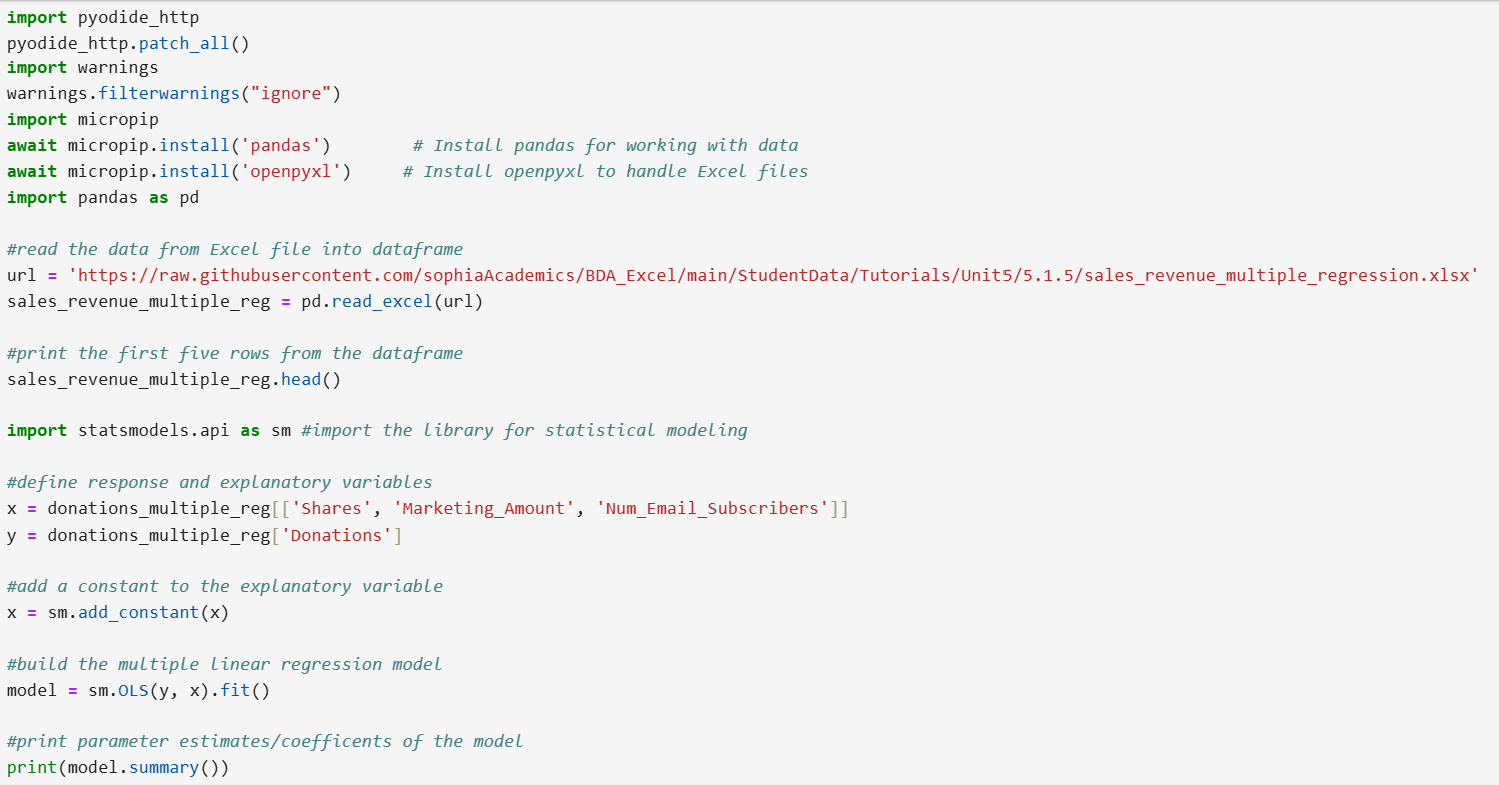
The summary of the regression model is provided below. Using the information highlighted in the orange, a hypothesis test will be conducted for each of the explanatory variables. A description of each of the columns in the highlighted output is provided below:

• coef (Coefficient): These are the values of the estimated coefficients for each explanatory variable in the model (the b’s).
• std err (Standard Error): Standard error for each explanatory variable.
• t (t-statistic): Ratio of the estimated coefficient to its standard error.
• P > | t | (p-value): The p-value that will be used to test whether each of the explanatory variables has a significant effect on the response variable or not.

The upcoming paragraphs will provide detailed explanations of each of these highlighted pieces of output and how they are used to perform the hypothesis tests.



Shares:

Step 1: State the Hypotheses.

• (no effect of number of social media shares on amount of donation; number of social media shares is not predictive of amount of donation)
• (number of social media shares does effect/is predictive of amount of donation)

Step 2: Gather the Data: The data has been imported from Excel into a pandas DataFrame.  

Step 3: Choose the Significance Level: Use a level of significance of

Step 4: Perform the t-test.

The t-test calculates a t-statistic which is:

The standard error of the coefficient is a measure of how precise the estimated coefficient is. It tells you how much the estimated coefficient would vary if you repeated the study with different samples. A smaller standard error means the estimate is more precise, while a larger standard error means the estimate is less precise.

The t-statistic is a number that helps you understand if an explanatory variable (number of social media shares) has a significant effect on the response variable (amount of donations). It tells you how far the estimated coefficient (the number that shows the relationship between the variables) is from zero, indicating whether the relationship is strong enough to be considered significant.

‘How far’ is significant?

• The further the t-statistic is from zero, the stronger the evidence against the null hypothesis (which states there is no effect). This means that the explanatory variable (number of social media shares) likely has a significant effect on the response variable (amount of donations)
• The closer the t-statistic is to zero, the weaker the evidence against the null hypothesis (which states there is no effect). This suggests that the observed data is more likely to have occurred by chance, indicating that the explanatory variable (number of social media shares) may not have a significant effect on the response variable (amount of donations).

How "far away" from zero does the t-statistic have to be for you to reject the null hypothesis? This is what the p-value tells you. 

• Small p-value (usually ≤ 0.05): If the p-value is less than 0.05, you reject the null hypothesis. This means there is strong evidence that the parameter is significantly different from zero, indicating that the explanatory variable (number of social media shares) has a significant effect on the response variable (amount of donations).
• Large p-value (usually > 0.05): If the p-value is greater than 0.05, you fail to reject the null hypothesis. This means there is not enough evidence to conclude that the parameter is significantly different from zero. In other words, the explanatory variable (number of social media shares) does not have a statistically significant effect on the response variable (amount of donations).

Step 5: Make a Decision.

Since the p-value for Shares (0.011) (level of significance of 0.05), you can reject the null hypothesis.

Step 6: Interpret the Results.

Since the p-value (0.011) is less than the significance level, you reject the null hypothesis. This means there is evidence that is significantly different from zero, indicating that the explanatory variable, the number of social media shares, has a significant effect on the response variable, the amount of donations. That is, the number of social media shares is predictive of the amount of donations the non-profit will receive.

Marketing_Amount:

Step 1: State the Hypotheses.

• (no effect of the amount spent on marketing on amount of donation; the amount spent on marketing is not predictive of the amount of donation)
• (amount spent on marketing does effect/is predictive of the amount of donation)

Step 2: Gather the Data: The data has been imported from Excel into a pandas DataFrame.  

Step 3: Choose the Significance Level: Use a level of significance of

Step 4: Perform the t-test.

Step 5: Make a Decision.

Since the p-value for Marketing_Amount (0.129) (level of significance), you fail to reject the null hypothesis. This means there is not enough evidence to conclude that is significantly different from zero, indicating that the amount spent on marketing does not have a statistically significant effect on the amount of donations the non-profit will receive.

Num_Email_Subscribers:

Step 1: State the Hypotheses.

• (no effect of the number of email subscribers on amount of donation; the number of email subscribers is not predictive of the amount of donation)
• (number of email subscribers does effect/is predictive of the amount of donation)

Step 2: Gather the Data: The data has been imported from Excel into a pandas DataFrame.  

Step 3: Choose the Significance Level: Use a level of significance of

Step 4: Perform the t-test.

Step 5: Make a Decision.

Since the p-value for Num_Email_Subscribers (0.189) (level of significance), you fail to reject the null hypothesis. This means there is not enough evidence to conclude that is significantly different from zero, indicating that the number of email subscribers does not have a statistically significant effect on the amount of donations the non-profit will receive.

Given the regression model indicates that the amount of spent on marketing for the fundraising campaigns (Marketing_Amount) and the number of email subscribers for each campaign (Num_Email_Subscribers) are not significant predictors of the amount of donations, the non-profit organization can still glean several practical insights:

• Focus on Social Media Engagement: Since Shares (number of social media shares) is a significant predictor, the organization should prioritize strategies that increase social media engagement. This could include creating more shareable content, running social media campaigns, and encouraging supporters to share posts.
• Reevaluate Marketing Spend: Since Marketing_Amount is not a significant predictor, the organization might reconsider its marketing budget allocation. They could explore more cost-effective marketing strategies or redirect funds to areas that have a proven impact on donations.
• Optimize Email Campaigns: Although Num_Email_Subscribers is not a significant predictor, the organization should analyze the content and frequency of their email campaigns. Improving the quality and targeting of emails might enhance their effectiveness, even if the sheer number of subscribers is not directly linked to donation amounts.

did you know

In regression hypothesis testing, you never conclude that the null hypothesis is true. The only two choices are to:

• Reject the null hypothesis.
• Fail to reject the null hypothesis.

Below is a list of key reasons as to why you do not conclude to accept the null hypothesis:

1. You start by assuming Hypothesis testing aims to find out if there is sufficient evidence to challenge and reject this assumption. 
2. Failing to reject means there is insufficient evidence to support that β is not zero. It does not confirm β is zero.
3. Hypothesis tests seek evidence against If evidence from the sample data is weak, you fail to reject but this does not prove is true.

Now it is your turn to practice interpreting the results of hypothesis testing for a multiple linear regression model!

try it

You are going to return to a similar example you have worked with previously, but now you are going to focus on the multiple regression output to determine which explanatory variables are important in predicting the response variable.

You are a data analyst working on an analytical project. Your task is to build a multiple linear regression model that can predict sales revenue based on several explanatory variables using Python.

You previously built a multiple linear regression model in Python to predict sales using the following explanatory variables:

• Sales_Revenue: The revenue generated from sales (in dollars) each month.
• Marketing_Spend: The amount of money spent on marketing (in dollars) each month.
• Customer_Reviews: Number of customer reviews left on a website like Google reviews each month.
• Sales_Team_Size: Number of sales team members for each month.

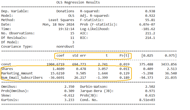
The output of the multiple regression model is provided below:



Perform the following:

1. Using the multiple regression output provided, conduct a hypothesis test for each explanatory variable. State the null and alternative hypotheses that are tested for each explanatory variable. Use a 0.05 level of significance (α) and make a concluding statement regarding whether the explanatory variable is useful/helpful in predicting sales based on the results of the hypothesis test.

Solution:

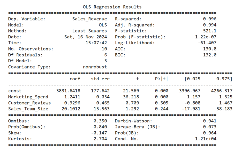
The part of the regression output you should focus on is highlighted below:



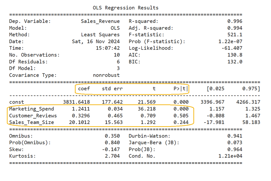Marketing_Spend

• 
• 

The p-value associated with Marketing_Spend is < 0.001 (the value 0.000 in the P>|t| column means the p-value is extremely small, less than 0.0001). Since the p-value is less than the level of significance (0.05), you can reject the null hypothesis and conclude that is not 0. That is the amount spent on marketing is predictive of sales revenue.

Customer_Reviews

• 
• 

The p-value associated with Customer_Reviews is 0.505, which is greater than the level of significance, α. Since the p-value is greater than the level of significance, you fail to reject the null hypothesis. This means there is not enough evidence to conclude that is significantly different from zero, indicating that the number of customer reviews is not predictive of sales revenue.

Sales_Team_Size

• 
• 

The p-value associated with Sales_Team_Size is 0.244, which is greater than the level of significance, α. Since the p-value is greater than the level of significance, you fail to reject the null hypothesis. This means there is not enough evidence to conclude that is significantly different from zero, indicating that the size of the sales team is not predictive of sales revenue.

watch

Check out this video on interpreting the results of hypothesis testing for a multiple linear regression model.

2c. Interpreting Standard Errors: Enhancing Regression Results Insights

Interpreting standard errors is essential for gaining deeper insights into regression results, as it helps determine the accuracy and dependability of the estimated relationships between variables.

Let's review standard errors in the context of sampling distributions, and then relate this concept to predicting donation amounts for a non-profit organization.

1. Sampling Distribution:

• When you take multiple samples from a population and calculate a statistic (for example, the mean) for each sample, you get a distribution of those statistics. This is called the sampling distribution.
• The sampling distribution shows how the statistic (for example, the mean) varies from sample to sample.

2. Sampling Distribution of the Regression Coefficients

• When you perform regression analysis, you estimate coefficients ( etc.) that describe the relationship between the explanatory variables and the response variable.
• If you were to take multiple samples from the population and calculate these coefficients for each sample, you would get a distribution of these coefficients. This is known as the sampling distribution of the regression coefficients.

The standard error of a regression coefficient measures the variability of that coefficient across different samples. It tells you how much the estimated coefficient is expected to vary due to random sampling.

• Small Standard Error: Indicates that the coefficient is estimated with high precision. The sampling distribution is narrow, meaning the coefficient does not vary much from sample to sample.
• Large Standard Error: Indicates that the coefficient is estimated with less precision. The sampling distribution is wider, meaning the coefficient varies more from sample to sample.

In your regression model where you have been predicting donation amounts, you have the following standard errors for your explanatory variables:

• Shares (Standard Error: 0.478):
  • A small standard error suggests that the coefficient for Shares is estimated with high precision. The sampling distribution of this coefficient is narrow, indicating that the number of social media shares is a reliable predictor of donation amounts.
• Marketing_Amount (Standard Error: 9.505):
  • A larger standard error indicates less precision in the estimate of the coefficient for Marketing_Amount. The sampling distribution is wider, suggesting that the effect of marketing amount on donations is more variable and less reliable as a predictor.
• Num_Email_Subscribers (Standard Error: 26.217):
  • An even larger standard error suggests that the coefficient for Num_Email_Subscribers is estimated with the least precision. The sampling distribution is very wide, indicating that the number of email subscribers may not be a strong or consistent predictor of donation amounts.