Impact of Price on Quantity Supplied/Demanded

1. Law of Demand: A Review

The law of demand is the inverse correlation between price and quantity, with all other variables being fixed.

For example, here is a demand schedule for Granny Smith apples outlining how many apples a consumer would purchase per week at various prices. At high prices, consumers do not want to purchase as many, while as the price falls, they want to purchase more.

Price of Granny Smith Apples	Quantity of Granny Smith Apples Each Week
$2.00	0
$1.75	1
$1.50	2
$1.25	3
$1.00	4
$0.75	5
$0.50	6
$0.25	7
$0.00	8

When we plot the points on a graph, we can see the inverse relationship between price and quantity, illustrated by a downward-sloping demand curve.

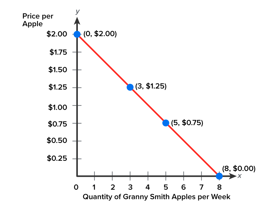
As the price of apples goes down, we buy more. As the price of apples goes up, we move along the curve to buy fewer apples.

Therefore, there is a negative relationship between price and quantity for demand.

hint

It is important to remember, though, that the idea of ceteris paribus, which means that everything else is held constant, applies in this situation. This assumes that only the price of Granny Smith apples has changed. Nothing else has changed, like the price of Gala apples, the price of oranges and bananas, or even a consumer’s income, because those things could certainly impact how many Granny Smith apples are purchased. We are only talking about buying more or less because the price of Granny Smith apples went up or down.

We refer to this as a movement along the curve as the price changes. As mentioned, as the price of Granny Smith apples drops, we buy more. This only involves a relationship between the two axes that comprise the graph—the price of Granny Smith apples and the quantity that is being purchased.

Therefore, we do not need a new demand curve. We simply move from one point to the next to show the price going up or down, which is why this is called movement along the demand curve.

hint

It is important to differentiate between a change in the quantity demanded and a change in demand itself. Often, people will make the mistake of inferring that since the price went up, demand went down. For demand to go down, this would require the whole curve to have a new relationship or for people to buy less at every single price, which is not the case here. Therefore, we say that as the price changes, it represents a change in the quantity demanded.

term to know

Law of Demand

The inverse correlation between price and quantity, with all other variables being fixed.

2. Law of Supply: A Review

The law of supply states that if the price of a good decreases, the quantity supplied decreases. The opposite would also be the case, meaning that as prices go up, the quantity supplied would also increase.

Again, using the same prices for apples, you can now see a different relationship between price and quantity.

Price of Granny Smith Apples	Quantity of Granny Smith Apples Each Week
$2.00	7
$1.75	6
$1.50	5
$1.25	4
$1.00	3
$0.75	2
$0.50	1
$0.25	0

As the price goes down, the quantity these farmers are willing to produce falls because, at very low prices, the farmers likely cannot even cover their costs. As the price goes up, they have a greater incentive, ability, and willingness to supply, so the quantity supplied rises.

This represents a positive relationship between price and quantity for supply.

hint

Again, the concept of ceteris paribus applies here. As the price of apples falls, we can expect farmers to produce fewer apples. Some of them may not want to produce apples anymore because they cannot cover their costs. With ceteris paribus, we are holding everything else constant, assuming that only the price of apples has changed. We are not changing the price of their resources or inputs, such as land, labor, or capital. We are not changing the technology used, which impacts how easy or difficult it is for them to produce. We are only changing the market price of apples.

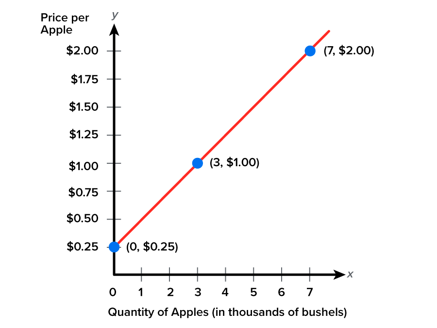
Again, a change in price will cause movements along the supply curve. As the price of Granny Smith apples increases, farmers want to supply more. This only involves a relationship between price and quantity, so we do not need a new curve. We simply move along the curve to see the new price and quantity combination.

hint

As the price goes up, the quantity supplied goes up, and as the price goes down, the quantity supplied goes down. We do not, however, say that the supply itself has changed.

term to know

Law of Supply

If the price of a good decreases, the quantity supplied decreases.

3. Finding Equilibrium

3a. At prices above $1.00: Q_s > Q_d

Now, if we look at these movements along the curve, you can see that at prices above $1 where these two curves converge, the quantity supplied exceeds the quantity demanded.

When that occurs, there is an incentive or a gap between the supply and demand curves.

In this case, there will be an incentive for grocers to lower the price. You may recall that as we lower the price, we simply move along the curve. We do not need a new curve.

So, as we lower the price, the quantity supplied would fall, the quantity demanded would rise, and they would meet in the middle.

If the price were too low, then there would be a gap, but the price is currently where the quantity demanded exceeds the quantity supplied, meaning that there are a lot of people buying but not a lot of people producing.

3b. At prices below $1.00: Q_d > Q_s

At prices below $1 where these two curves converge, the quantity demanded exceeds the quantity supplied.

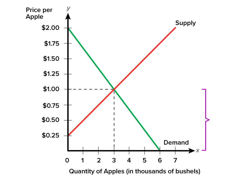
As grocers raise the price, we see the quantity demanded fall and, at the same time, we see the quantity supplied rise—according to the laws of supply and demand—until we meet in the middle at equilibrium.

3c. At the prices of $1.00: Q_s = Q_d

The equilibrium price is the only price where there is no tendency for change, and it is the only price that clears the market, where the quantity supplied equals exactly the quantity demanded.

Therefore, equilibrium is defined as the price and quantity pair at which supply and demand intersect; in other words, it is the price and quantity at which the market clears.

term to know

Equilibrium

The price and quantity pair at which supply and demand intersect—that is, the price and quantity at which the market clears.