Table of Contents |
If you recall from a previous lesson, normal distributions have density curves that are symmetric and bell-shaped. The mean, median, and mode of the normal distribution are all the same and equal to the center value of the density curve. However, there are situations in which, unlike normal distributions, a distribution may not be symmetrical. We call these skewed distributions.
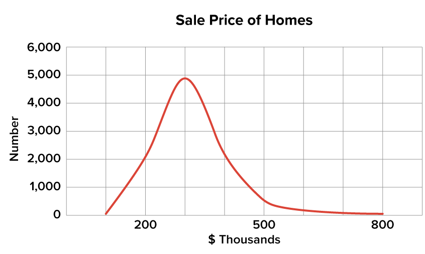
The first distribution that you see below is skewed. It reflects a situation in which there would be many values concentrated toward the lower end of the distribution relative to the higher end. This is typically how the home values are distributed.
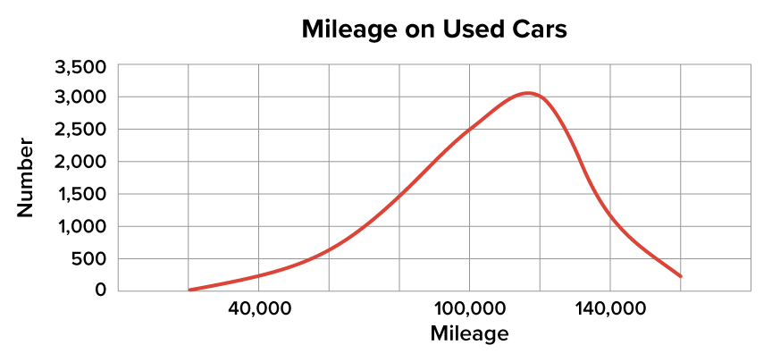
This second distribution is skewed, and it reflects a situation in which there will be many values concentrated toward the higher end of the distribution relative to the lower end. A good example of this distribution would be the mileage on the odometers of used cars.
Refer back to the home values graph. On the bottom (horizontal) axis, you have the price listed in thousands of dollars. The range is from around $100,000 up to almost $800,000. The majority of the values are concentrated right around the $300,000 mark. This is a right-skewed, or positively skewed, distribution curve.
Why is it right-skewed? Because so many observations are around that $300,000 point, but there are also a lot of homes priced much higher. That pulls the mean up while leaving the median or the middle value relatively low.
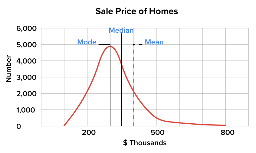
In this case, the mode would be the smallest value, then the median, and then the mean. You’d read the graph along the horizontal axis from left to right.
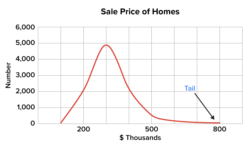
When you look at a right-skewed distribution, the far right-hand side is pointing to the right. Imagine it’s an arrow, with the tail indicating the direction of the skew.
The mean is $400,000, which is higher than either the median ($325,000) or the mode ($300,000). This is a key indicator of a right-, or a positively, skewed distribution.
A left-skewed distribution, on the other hand, would be an example such as the mileage on used cars. If you look at the distribution of the mileage of used cars shown below, you notice that there are similarities to the previous graph. However, it’s not going to necessarily look exactly the same. This type of distribution is called a left-skewed distribution, or a negatively skewed distribution.
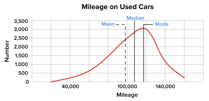
In left-skewed distributions, including this one, the mode is greater than the median, and the median is greater than the mean.
Mode = 118,000 miles
Median = 108,000 miles
Mean = 97,000 miles
You see a relatively low number on the lower end in terms of the value of miles on a car. This is because people might wait a lot longer to trade in their vehicles, which might mean they have higher mileage. You’d see a left-skewed distribution. Notice that the tail points to the left.
Source: THIS TUTORIAL WAS AUTHORED BY DAN LAUB FOR SOPHIA LEARNING. PLEASE SEE OUR TERMS OF USE.