Use Sophia to knock out your gen-ed requirements quickly and affordably. Learn more
×

Identifying Missing Data

Author: Sophia

what's covered
In this lesson, you will learn how to identify and remedy missing data in Excel. Specifically, this lesson will cover:

Table of Contents

1. Identifying Missing Data

In earlier tutorials, we emphasized the significance of addressing missing data. If missing data is not identified and remedied, it can introduce inaccuracies in the results based on the analysis. Identifying missing data allows us to choose the appropriate method to remedy the missing data. When possible, you want to impute, meaning fill in, missing values in an effort to prevent the deletion of a row or observation from your data set.

How do we resolve missing data to avoid losing it and potentially creating bias during analysis?

1a. Identifying Missing Data in Excel

Identifying missing data in Excel can be performed in several ways. You will explore two effective techniques in this section. One method involves using an Excel formula, and one method uses filtering to detect missing values.

As you look across the data columns in the Netflix data file, you observe that there are missing values scattered throughout the columns.

EXAMPLE

You can use the Excel COUNTIFS() function to detect if a particular column contains missing values. For instance, using COUNTIFS() you can determine that there are 27 missing values in the director column.

try it
Use the COUNTIFS() function to determine the number of missing values for the director column in the Netflix data.

1. Open the netflix.xlsx file.

2. Create a new column in column P. Name your new column missing_director, using the header row (Cell P1).

The COUNTIFS function in Excel allows you to count the values in a column that meet a certain criterion. The general form of the formula is:

=COUNTIFS(range, criteria)
The first argument is the range of cells. The second argument is the criteria to be included in the count. If you want to specify missing values, use the criteria “” (two double quotes with no spaces).

3. In cell P2, enter the following formula:

=COUNTIFS(H2:H101,“”)
The director column is in column D, and the rows range from row 2 to row 101. This formula returns the value 27; the director column has 27 missing values.

watch
Follow along with this video to determine the number of missing values using the COUNTIFS function.

The next example will show you how to filter to determine if a column contains missing values.

EXAMPLE

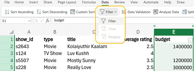
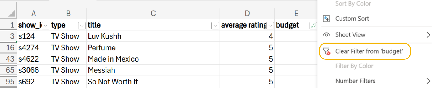
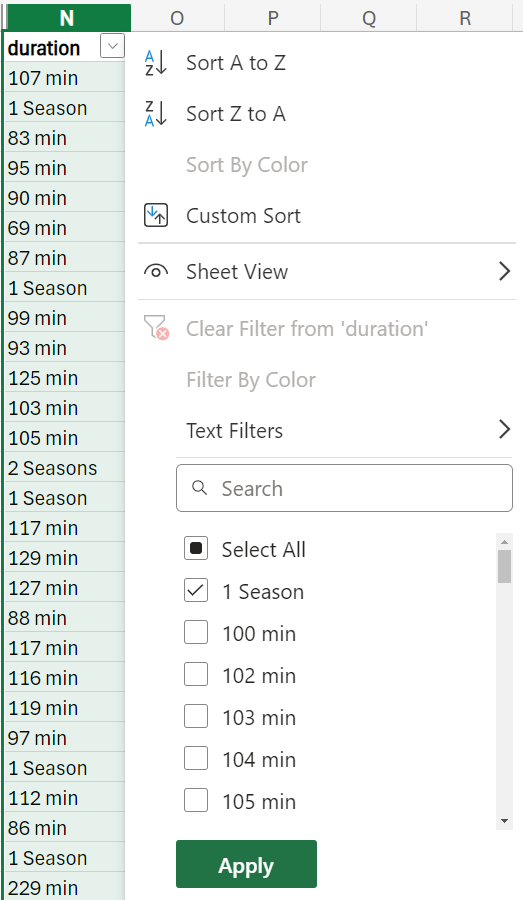
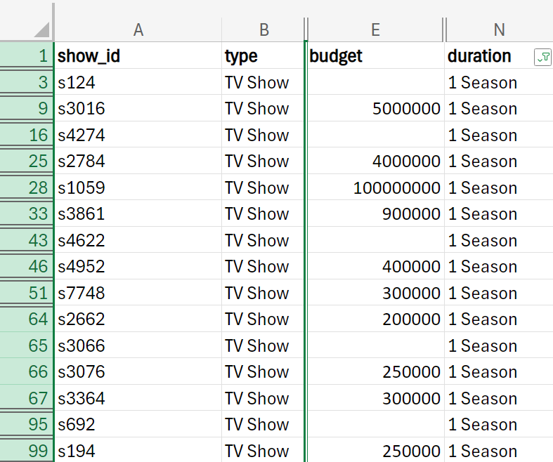
Using a filter, you can determine the number of missing values in the budget column. The filter result, shown below, returns five missing values.

try it
Let’s determine the number of missing values in the budget column.

Open the netflix.xlsx data and perform the following:

  1. Select all the rows in the budget column.
  2. In the Data menu select Filter.


  3. Use the drop-down arrow that now appears in the budget column.
  4. Deselect the Select All checkbox to remove all the checks from the values and then check the box for Blanks to return only the rows where budget is blank (missing).


  5. Select Apply. The worksheet will be updated to show only the five rows where the value of budget is missing. Check that your sheet looks like the one in the example image.
  6. To revert to viewing all the rows in the data, clear the filter from the budget column by selecting the drop-down arrow in the budget column and selecting Clear Filter from ‘budget.’


  7. To remove the filter entirely from the budget column, select Data from the ribbon, then FilterClear. You will notice the filter icon in the column header is now removed from the budget column.

watch
Follow along with this video to determine the number of missing values using a filter.


2. Remedying Missing Data

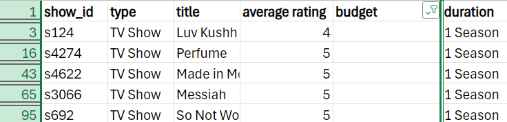
Once you have detected that you have missing values, you then must decide what to do with the missing values. While ultimately how you handle the missing values depends largely on the context of the business scenario, in most circumstances, you will want to handle the missing values in some manner rather than just deleting the observations with the missing values. In the next section, we will make some presumptions about the analysis goals of the Netflix data to illustrate how you can use Excel to remedy the missing values you have detected.

2a. Remedying Missing Data In Excel

You have just determined that the director column has 27 missing values. Approximately 30% of this column has missing values. Under a circumstance like this, you would not want to ignore the missing values. If you worked at Netflix or wanted to invest the time, you could impute the missing values by finding the directors of the 27 titles that are missing. Let’s presume you do not want to invest this amount of time. For example, suppose you were going to create a report related to the director column. You do not want missing values in the report because you want the report to look professional. So, you are going to impute the missing values with the value “Unknown.” This way, the data will no longer be missing, and the imputed value represents a true characterization of your knowledge of the missing director's values.

EXAMPLE

You can use a combination of the IF() and ISBLANK() functions to impute the missing values of the director column with the value “Unknown.” You can create a new column, director_no_miss that contains the imputed values of the director.

try it
Impute the missing values of the director column with the value “Unknown.”

Open netflix.xlsx data and perform the following:

1. Create a new column named director_no_miss in column R of the Excel worksheet.

2. In cell R2, enter the formula:

=IF(ISBLANK(H2), “Unknown”,H2)
This formula checks if the cell in column H (the director column) is missing. If the value of director is missing, it imputes the value “Unknown.” If the director column is not missing, it retains the original director's name.

3. Once you have your formula in the first cell of the director_no_miss column, hover over the small black plus sign (Auto-Fill Handle) at the bottom-right corner of the cell. Click and hold the left mouse button, then drag the handle down to the last cell where you want the formula to apply. (R101)

4. Check your work by comparing the imputed values of the director column to those in the example above.

EXAMPLE

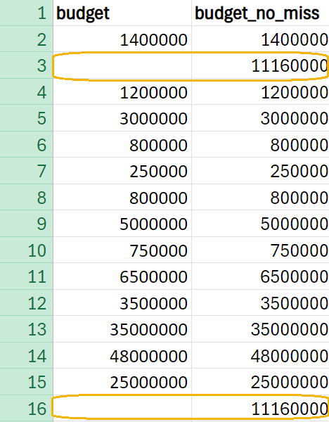
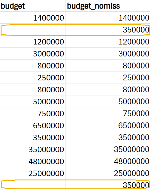
You can use Excel to impute missing values for a quantitative variable as well. In a previous example, you determined that five TV shows that lasted 1 Season had missing values for budget.


You can use Excel formulas to impute the missing values using the median of the budget column for TV Shows that lasted for 1 Season.

try it
Impute the missing values of budget with the median of TV Shows that lasted 1 Season.

Remember that the missing values for budget are all related to TV Shows that had a duration of 1 Season.

Suppose you imputed these missing values with the median of the budget column. You would need to be careful because the missing values are for only one category of type and duration (TV shows that lasted 1 Season). TV shows that lasted 1 Season will have a different budget than TV shows that lasted for 2 seasons, 3 seasons, and so on. So, you would not want to impute the missing values with the median of the budget column using all the data. Rather, impute the missing value of budget with the subset of data for TV Shows that lasted 1 Season.

To impute the missing values for budget, you need to find the median budget amount for the TV shows that lasted 1 Season and use this as your imputed value.

To impute the missing values of budget with the median of TV Shows that lasted 1 Season, perform the following.

1. Apply a filter to the duration column by selecting all the rows of the duration column and then select Home menu → Sort and FilterFilter.

2. Select the drop-down arrow that appears in the duration column.

3. Select the Select All checkbox to remove all the checks from the values and then check the box for 1 Season to filter all rows where the title's duration is 1 Season.


4. Select Apply. The worksheet will be updated to show all the rows where the value of duration is 1 Season.


You can now find the median for the budget for this subset of data that represents TV shows that were 1 Season.

When you calculate the median of the budget column for this subset of data, you need to use the SUBTOTAL() function along with an array formula. An array formula in Excel is a type of formula that operates on multiple values simultaneously, rather than just a single value.

First, let’s describe the SUBTOTAL() function.

The SUBTOTAL() function allows you to calculate a summary statistic of only the visible cells in the worksheet. In Excel, SUBTOTAL() has the general form:

=SUBTOTAL(function_num, range)
Suppose you wanted to calculate the average of the budget column for this subset of data. The function_num argument is a numeric value that specifies what type of summary statistic you wish to apply. For example, ‘1’ corresponds to the average. The range argument is the range of the cells you want to average.

5. In a blank cell, say E114, enter the following formula to find the average of the budget column for TV Shows that lasted 1 Season and then select ENTER.

=SUBTOTAL(1,E3:E99)
This equation should return the number 11160000.

Keep in mind that averages can be skewed by outliers, which is why this average appears inflated. This is why you are not going to impute with the average. The average is influenced by outliers. If you have known outliers in your data, it is better to impute with the median.

The SUBTOTAL() function does not support median calculation. To calculate the median of filtered rows, you use the AGGREGATE() function, which works in a similar manner as SUBTOTAL() when performing operations on filtered rows.

6. In a blank cell, say E117, type the following formula to find the median of the budget column for TV Shows that lasted 1 Season and then select ENTER.

=AGGREGATE(12,5,E3:E99)
The value 12 specifies the median calculation, and 5 tells Excel to ignore hidden (filtered out) rows.

E3:E99 is the range of the data in the filtered worksheet.

The median of filtered data is $350,000. You will see this value is much smaller than the average of the filtered data, which was $11,160,000, because the median is the middle number of the budget values. The median does not consider those extremely large budget values in the data.

You are now ready to impute the missing values of budget using the median of the TV Shows that lasted 1 Season. You are going to perform a similar task as when you imputed the missing values for the budget column.

7. Remove the filter from the duration column by selecting the drop-down arrow in the duration column and selecting Clear Filter from ‘duration’Apply.

8. Create a new column named budget_no_miss in column S of the Excel worksheet.

9. In cell S2, type the following formula.

=IF(ISBLANK(E2),350000,E2)
10. This formula checks if the cell in column E (the budget column) is missing. If the value of budget is missing, it imputes the value 350000 (the median of the TV Shows that lasted 1 Season that was found in previous steps). If the budget column is not missing, it retains the original budget value.

11. Once you have your formula in the first cell of the budget_no_miss column, hover over the small black plus sign (Auto-Fill Handle) at the bottom-right corner of the cell. Click and hold the left mouse button, then drag the handle down to the last cell where you want the formula to apply.

The first 15 rows of budget_no_miss should look like the following:


12. Check your work by comparing the imputed values of the budget column to the example.

watch
Follow along with these videos to impute missing values with the median value.

try it
How would you remedy the missing values in from the Fraudulent transaction data set?


Identify the technique you might use to address each instance of missing data.
  • Transaction_Date: This is a categorical variable, so you could impute with the mode (the most frequently occurring date in the data). If appropriate resources were available at your company, you could attempt to impute the transaction date by using a domain-specific method by determining if IT could determine the transaction date given the customer’s IP address.
  • Transaction_Type: This is a categorical variable, so you could impute with the mode.
  • IP_Address: Domain-specific imputation. Since you have a unique customer identifier (Customer_ID), you can see if User_ID 104 has another transaction in another data set and use the IP address from another User_ID 104’s transactions.
  • Location: This is a categorical variable, so you could impute with the mode. Or, again, if resources are available, use the customer’s IP address to determine the location to perform domain-specific imputation.

think about it
What if there were other subsets of data that were missing for the budget column in the Netflix data? For instance, what if there were several missing values for movie titles in addition to the missing values for TV Shows that lasted 1 Season? How would you modify the Excel functions you have learned in this tutorial to impute the missing values for different subsets of the budget column?

term to know
Array Formula
Performs calculations on multiple values (values in rows and columns) simultaneously in Excel.

summary
In this lesson, you learned how to identify and remedy missing data in Excel and discussed the importance of addressing these gaps to avoid inaccuracies in analysis results. The lesson emphasized that handling missing values depends on the business context, but it is generally better to address them rather than delete affected observations. Practical methods for remedying missing data were demonstrated using a real-world Netflix dataset. You also learned how to impute missing values based on the analysis goals of the dataset. This lesson was built on earlier tutorials that highlighted the significance of managing missing data effectively.

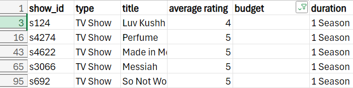
Source: THIS TUTORIAL WAS AUTHORED BY SOPHIA LEARNING. PLEASE SEE OUR TERMS OF USE.

Terms to Know
Array Formula

Performs calculations on multiple values (values in rows and columns) simultaneously in Excel.