Table of Contents |
Suppose a pharmaceutical company manufactures ibuprofen pills. They need to perform some quality assurance to ensure they have the correct dosage, which is supposed to be 500 milligrams. This is a two-sided test because if the company's pills are deviating significantly in either direction, meaning there are more than 500 milligrams or less than 500 milligrams, this will indicate a problem.

In a random sample of 125 pills, there is an average dose of 499.3 milligrams with a standard deviation of 6 milligrams. Because this is quantitative data, 500 mg is the population mean. We can use the following formula to calculate the z-score:

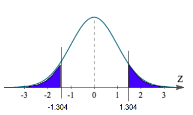
We get a z-score of negative 1.304. Because this is a two-sided test, it is not enough to just look at the left tail. We also have to look at the equivalent of the right tail, or a positive 1.304.
Now that we have the z-score, we can use a variety of methods to find the probability, or p-value.
The first way to find the p-value is to use the z-table. In the z-table, the left column will show values to the tenths place, while the top row will show values to the hundredths place. If we have a z-score of -1.304, we need to round this to the hundredths place, or -1.30. In the left column, we will first find the tenths place, or -1.3. In the top row, we will find the hundredths place, or 0.
| z | 0.00 | 0.01 | 0.02 | 0.03 | 0.04 | 0.05 | 0.06 | 0.07 | 0.08 | 0.09 |
|---|---|---|---|---|---|---|---|---|---|---|
| -3.4 | 0.0003 | 0.0003 | 0.0003 | 0.0003 | 0.0003 | 0.0003 | 0.0003 | 0.0003 | 0.0003 | 0.0002 |
| -3.3 | 0.0005 | 0.0005 | 0.0005 | 0.0004 | 0.0004 | 0.0004 | 0.0004 | 0.0004 | 0.0004 | 0.0003 |
| -3.2 | 0.0007 | 0.0007 | 0.0006 | 0.0006 | 0.0006 | 0.0006 | 0.0006 | 0.0005 | 0.0005 | 0.0005 |
| -3.1 | 0.0010 | 0.0009 | 0.0009 | 0.0009 | 0.0008 | 0.0008 | 0.0008 | 0.0008 | 0.0007 | 0.0007 |
| -3.0 | 0.0013 | 0.0013 | 0.0013 | 0.0012 | 0.0012 | 0.0011 | 0.0011 | 0.0011 | 0.0010 | 0.0010 |
| -2.9 | 0.0019 | 0.0018 | 0.0017 | 0.0017 | 0.0016 | 0.0016 | 0.0015 | 0.0015 | 0.0014 | 0.0014 |
| -2.8 | 0.0026 | 0.0025 | 0.0024 | 0.0023 | 0.0023 | 0.0022 | 0.0021 | 0.0021 | 0.0020 | 0.0019 |
| -2.7 | 0.0035 | 0.0034 | 0.0033 | 0.0032 | 0.0031 | 0.0030 | 0.0029 | 0.0028 | 0.0027 | 0.0026 |
| -2.6 | 0.0047 | 0.0045 | 0.0044 | 0.0043 | 0.0041 | 0.0040 | 0.0039 | 0.0038 | 0.0037 | 0.0036 |
| -2.5 | 0.0062 | 0.0060 | 0.0059 | 0.0057 | 0.0055 | 0.0054 | 0.0052 | 0.0051 | 0.0049 | 0.0048 |
| -2.4 | 0.0082 | 0.0080 | 0.0078 | 0.0075 | 0.0073 | 0.0071 | 0.0069 | 0.0068 | 0.0066 | 0.0064 |
| -2.3 | 0.0107 | 0.0104 | 0.0102 | 0.0099 | 0.0096 | 0.0094 | 0.0091 | 0.0089 | 0.0087 | 0.0084 |
| -2.2 | 0.0139 | 0.0136 | 0.0132 | 0.0129 | 0.0125 | 0.0122 | 0.0119 | 0.0116 | 0.0113 | 0.0110 |
| -2.1 | 0.0179 | 0.0174 | 0.0170 | 0.0166 | 0.0162 | 0.0158 | 0.0154 | 0.0150 | 0.0146 | 0.0143 |
| -2.0 | 0.0228 | 0.0222 | 0.0217 | 0.0212 | 0.0207 | 0.0202 | 0.0197 | 0.0192 | 0.0188 | 0.0183 |
| -1.9 | 0.0287 | 0.0281 | 0.0274 | 0.0268 | 0.0262 | 0.0256 | 0.0250 | 0.0244 | 0.0239 | 0.0233 |
| -1.8 | 0.0359 | 0.0351 | 0.0344 | 0.0336 | 0.0329 | 0.0322 | 0.0314 | 0.0307 | 0.0301 | 0.0294 |
| -1.7 | 0.0446 | 0.0436 | 0.0427 | 0.0418 | 0.0409 | 0.0401 | 0.0392 | 0.0384 | 0.0375 | 0.0367 |
| -1.6 | 0.0548 | 0.0537 | 0.0526 | 0.0516 | 0.0505 | 0.0495 | 0.0485 | 0.0475 | 0.0465 | 0.0455 |
| -1.5 | 0.0668 | 0.0655 | 0.0643 | 0.0630 | 0.0618 | 0.0606 | 0.0594 | 0.0582 | 0.0571 | 0.0559 |
| -1.4 | 0.0808 | 0.0793 | 0.0778 | 0.0764 | 0.0749 | 0.0735 | 0.0721 | 0.0708 | 0.0694 | 0.0681 |
| -1.3 | 0.0968 | 0.0951 | 0.0934 | 0.0918 | 0.0901 | 0.0885 | 0.0869 | 0.0853 | 0.0838 | 0.0823 |
| -1.2 | 0.1151 | 0.1131 | 0.1112 | 0.1093 | 0.1075 | 0.1056 | 0.1038 | 0.1020 | 0.1003 | 0.0985 |
| -1.1 | 0.1357 | 0.1335 | 0.1314 | 0.1292 | 0.1271 | 0.1251 | 0.1230 | 0.1210 | 0.1190 | 0.1170 |
| -1.0 | 0.1587 | 0.1562 | 0.1539 | 0.1515 | 0.1492 | 0.1469 | 0.1446 | 0.1423 | 0.1401 | 0.1379 |
This results in a p-value of 0.0968, or 9.68%, for a z-score of negative 1.304. We also need to take the positive 1.304 into account, which is the upper right tail.
To calculate the true p-value, we just need to multiply 0.0968 by two, or 0.1936. This would be a p-value of 19.36%.
The second method is using a graphing calculator. This can give us a more exact number because we will not have to cut off the z-score at the hundredths place. On the calculator, click "2nd," then "DISTR" for distribution. We will use "normalcdf," which stands for normal cumulative density function. When inserting the values into the calculator, we always go lower boundary to upper boundary.
In this case, the lower boundary was shaded all the way to the left of the curve, which would be negative infinity. We cannot enter negative infinity in our calculator, so instead, we can just enter negative 99. The shading stops at -1.304, so this is the upper boundary.
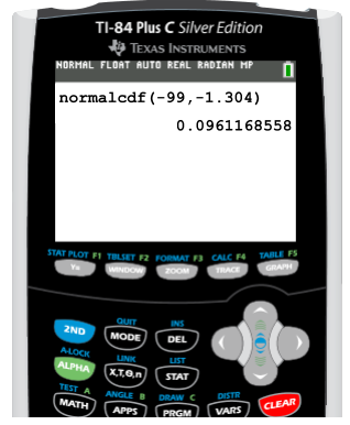
We get a value of 0.0961, which is about the same value as we got in the table. Again, we need to take both tails into account, so we can simply multiply this value by two to get a p-value of 0.1922, or 19.22%.
The third method to find the p-value is to use Excel. First, select "Formulas," choose the "Statistical" option, and pick "NORM.DIST." The first value we are going to input is the mean of the sample, which was 499.3, then the population mean which we are testing against, or 500, and finally the standard deviation, which was 6, divided by the square root of the sample of n. We can find the square root under the "Math and Trigonometry" option in "Formulas." The last value that we need to enter is "TRUE."
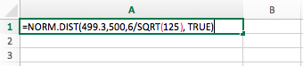
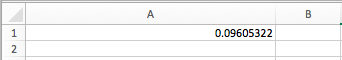
We get about the same value as we did with the table and the calculator. Since this is a two-sided test, we need to multiply the value by two, or 0.096 times two equals 0.1912.
In this next example, we'll look at the proportion of students who suffer from test anxiety. We want to test the claim that fewer than half of students suffer from test anxiety.

In this case, we will have a left-tailed test. Because this is qualitative data, meaning the students answer yes or no to suffering from test anxiety, this is a population proportion, and we can use the following formula to calculate the z-test statistic:

In a random sample of 1,000 students, 450 students claimed to have test anxiety. This will be p-hat, or the sample proportion. We can calculate this by dividing 450 by 1,000, or 0.45. The population proportion, p, is 50%, or 0.50. The complement of p, or q, can be found by calculating 1 minus 0.50, or 0.50. The sample size is 1,000.

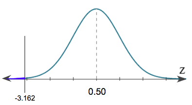
The corresponding z-score is negative 3.162. Testing against that half, or 50%, of students suffer from test anxiety, we get the following shaded region all the way to the left of our curve:
The first way to find the p-value is with the z-table. Remember, we can only go up to the hundredths place, so we will need to round -3.162 to -3.16. In the left column, we will first find the tenths place, or -3.1. In the top row, we will find the hundredths place, or 0.06.
| z | 0.00 | 0.01 | 0.02 | 0.03 | 0.04 | 0.05 | 0.06 | 0.07 | 0.08 | 0.09 |
|---|---|---|---|---|---|---|---|---|---|---|
| -3.4 | 0.0003 | 0.0003 | 0.0003 | 0.0003 | 0.0003 | 0.0003 | 0.0003 | 0.0003 | 0.0003 | 0.0002 |
| -3.3 | 0.0005 | 0.0005 | 0.0005 | 0.0004 | 0.0004 | 0.0004 | 0.0004 | 0.0004 | 0.0004 | 0.0003 |
| -3.2 | 0.0007 | 0.0007 | 0.0006 | 0.0006 | 0.0006 | 0.0006 | 0.0006 | 0.0005 | 0.0005 | 0.0005 |
| -3.1 | 0.0010 | 0.0009 | 0.0009 | 0.0009 | 0.0008 | 0.0008 | 0.0008 | 0.0008 | 0.0007 | 0.0007 |
| -3.0 | 0.0013 | 0.0013 | 0.0013 | 0.0012 | 0.0012 | 0.0011 | 0.0011 | 0.0011 | 0.0010 | 0.0010 |
| -2.9 | 0.0019 | 0.0018 | 0.0017 | 0.0017 | 0.0016 | 0.0016 | 0.0015 | 0.0015 | 0.0014 | 0.0014 |
| -2.8 | 0.0026 | 0.0025 | 0.0024 | 0.0023 | 0.0023 | 0.0022 | 0.0021 | 0.0021 | 0.0020 | 0.0019 |
This gives us a p-value of 0.0008, or 0.08%.
To find the p-value on the graphing calculator, click "2nd," then "DISTR" for distribution. Again, we will use "normalcdf." When inserting the values into the calculator, remember we always go lower boundary to upper boundary. In this case, the lower boundary was shaded all the way to the left of the curve, which would be negative infinity. We cannot enter negative infinity in our calculator, so instead, we can just enter negative 99. The shading stops at -3.162, so this is the upper boundary.
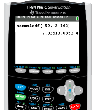
This answer shows a p-value of 0.00078, or 0.078%.
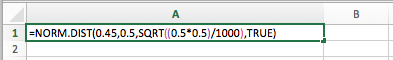
In Excel, select "Formulas," choose the "Statistical" option, and pick "NORM.DIST." The first value we are going to input is the sample proportion, "0.45," then the population proportion, "0.50," and finally the standard deviation, which was the square root of pq divided by n, or 0.50 times 0.50, divided by 1000. We can find the square root under the "Math and Trigonometry" option in "Formulas." The standard deviation should be input as "SQRT((0.50*0.50)/1000)." The last value that we need to enter is "TRUE."
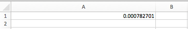
We get about the same p-value as we did with the z-table and the calculator.
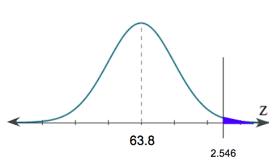
In this final example, we will be testing the claim that women in a certain town are taller than the average U.S. height, which is 63.8 inches.

From a random sample of 50 women, we get an average height of 64.7 inches with a standard deviation of 2.5 inches. Inches is a quantitative variable; therefore, the 63.8 inches is a population mean. We will then use the following formula to calculate the z-score:

We get a z-score of 2.546, which is labeled on the following distribution:
The first way to find the p-value is to use the z-table. In the z-table, the left column will show values to the tenths place, while the top row will show values to the hundredths place. If we have a z-score of 2.546, we need to round this to the hundredths place, or 2.55. In the left column, we will first find the tenths place, or 2.5. In the top row, we will find the hundredths place, or 0.05.
| z | 0.00 | 0.01 | 0.02 | 0.03 | 0.04 | 0.05 | 0.06 | 0.07 | 0.08 | 0.09 |
|---|---|---|---|---|---|---|---|---|---|---|
| 0.0 | 0.5000 | 0.5040 | 0.5080 | 0.5120 | 0.5160 | 0.5199 | 0.5239 | 0.5279 | 0.5319 | 0.5359 |
| 0.1 | 0.5398 | 0.5438 | 0.5478 | 0.5517 | 0.5557 | 0.5596 | 0.5636 | 0.5675 | 0.5714 | 0.5753 |
| 0.2 | 0.5793 | 0.5832 | 0.5871 | 0.5910 | 0.5948 | 0.5987 | 0.6026 | 0.6064 | 0.6103 | 0.6141 |
| 0.3 | 0.6179 | 0.6217 | 0.6255 | 0.6293 | 0.6331 | 0.6368 | 0.6406 | 0.6443 | 0.6480 | 0.6517 |
| 0.4 | 0.6554 | 0.6591 | 0.6628 | 0.6664 | 0.6700 | 0.6736 | 0.6772 | 0.6808 | 0.6844 | 0.6879 |
| 0.5 | 0.6915 | 0.6950 | 0.6985 | 0.7019 | 0.7054 | 0.7088 | 0.7123 | 0.7157 | 0.7190 | 0.7224 |
| 0.6 | 0.7257 | 0.7291 | 0.7324 | 0.7357 | 0.7389 | 0.7422 | 0.7454 | 0.7486 | 0.7517 | 0.7549 |
| 0.7 | 0.7580 | 0.7611 | 0.7642 | 0.7673 | 0.7704 | 0.7734 | 0.7764 | 0.7794 | 0.7823 | 0.7852 |
| 0.8 | 0.7881 | 0.7910 | 0.7939 | 0.7967 | 0.7995 | 0.8023 | 0.8051 | 0.8078 | 0.8106 | 0.8133 |
| 0.9 | 0.8159 | 0.8186 | 0.8212 | 0.8238 | 0.8264 | 0.8289 | 0.8315 | 0.8340 | 0.8365 | 0.8389 |
| 1.0 | 0.8413 | 0.8438 | 0.8461 | 0.8485 | 0.8508 | 0.8531 | 0.8554 | 0.8577 | 0.8599 | 0.8621 |
| 1.1 | 0.8643 | 0.8665 | 0.8686 | 0.8708 | 0.8729 | 0.8749 | 0.8770 | 0.8790 | 0.8810 | 0.8830 |
| 1.2 | 0.8849 | 0.8869 | 0.8888 | 0.8907 | 0.8925 | 0.8944 | 0.8962 | 0.8980 | 0.8997 | 0.9015 |
| 1.3 | 0.9032 | 0.9049 | 0.9066 | 0.9082 | 0.9099 | 0.9115 | 0.9131 | 0.9147 | 0.9162 | 0.9177 |
| 1.4 | 0.9192 | 0.9207 | 0.9222 | 0.9236 | 0.9251 | 0.9265 | 0.9279 | 0.9292 | 0.9306 | 0.9319 |
| 1.5 | 0.9332 | 0.9345 | 0.9357 | 0.9370 | 0.9382 | 0.9394 | 0.9406 | 0.9418 | 0.9429 | 0.9441 |
| 1.6 | 0.9452 | 0.9463 | 0.9474 | 0.9484 | 0.9495 | 0.9505 | 0.9515 | 0.9525 | 0.9535 | 0.9545 |
| 1.7 | 0.9554 | 0.9564 | 0.9573 | 0.9582 | 0.9591 | 0.9599 | 0.9608 | 0.9616 | 0.9625 | 0.9633 |
| 1.8 | 0.9641 | 0.9649 | 0.9656 | 0.9664 | 0.9671 | 0.9678 | 0.9686 | 0.9693 | 0.9699 | 0.9706 |
| 1.9 | 0.9713 | 0.9719 | 0.9726 | 0.9732 | 0.9738 | 0.9744 | 0.9750 | 0.9756 | 0.9761 | 0.9767 |
| 2.0 | 0.9772 | 0.9778 | 0.9783 | 0.9788 | 0.9793 | 0.9798 | 0.9803 | 0.9808 | 0.9812 | 0.9817 |
| 2.1 | 0.9821 | 0.9826 | 0.9830 | 0.9834 | 0.9838 | 0.9842 | 0.9846 | 0.9850 | 0.9854 | 0.9857 |
| 2.2 | 0.9861 | 0.9864 | 0.9868 | 0.9871 | 0.9875 | 0.9878 | 0.9881 | 0.9884 | 0.9887 | 0.9890 |
| 2.3 | 0.9893 | 0.9896 | 0.9898 | 0.9901 | 0.9904 | 0.9906 | 0.9909 | 0.9911 | 0.9913 | 0.9916 |
| 2.4 | 0.9918 | 0.9920 | 0.9922 | 0.9925 | 0.9927 | 0.9929 | 0.9931 | 0.9932 | 0.9934 | 0.9936 |
| 2.5 | 0.9938 | 0.9940 | 0.9941 | 0.9943 | 0.9945 | 0.9946 | 0.9948 | 0.9949 | 0.9951 | 0.9952 |
| 2.6 | 0.9953 | 0.9955 | 0.9956 | 0.9957 | 0.9959 | 0.9960 | 0.9961 | 0.9962 | 0.9963 | 0.9964 |
| 2.7 | 0.9965 | 0.9966 | 0.9967 | 0.9968 | 0.9969 | 0.9970 | 0.9971 | 0.9972 | 0.9973 | 0.9974 |
| 2.8 | 0.9974 | 0.9975 | 0.9976 | 0.9977 | 0.9977 | 0.9978 | 0.9979 | 0.9979 | 0.9980 | 0.9981 |
| 2.9 | 0.9981 | 0.9982 | 0.9982 | 0.9983 | 0.9984 | 0.9984 | 0.9985 | 0.9985 | 0.9986 | 0.9986 |
This gives us a p-value of 0.9946, or 99.46%.
However, when we are performing an upper-tailed test, or right-tailed test, that p-value from the table always reads left to right for our distribution. The p-value of 99.46% is associated with the 99.46% that is unshaded.
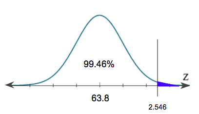
To get the percent that is shaded under the curve, we just need to calculate 100% minus 99.46%. This gives us the p-value of 0.54%, or 0.0054.
On the graphing calculator, again, we are going to click "2nd," then "DISTR," and use "normalcdf." When inserting the values into the calculator, remember we always go lower boundary to upper boundary of the shaded region. In this case, the lower boundary of the shaded region is our z-score, 2.546. The upper boundary goes all the way up to positive, but we cannot type positive infinity in our calculator. Instead, we can just enter positive 99.
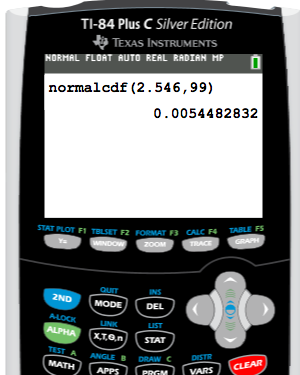
This answer shows a p-value of 0.0054, or 0.54%.
In Excel, first, select "Formulas," choose the "Statistical" option, and again pick "NORM.DIST." The first value we are going to input is the mean of the sample, which was 64.7, then the population mean which we are testing against, or 63.8, and finally the standard deviation, which was 2.5, divided by the square root of the sample size of 50. We can find the square root under the "Math and Trigonometry" option in "Formulas." The last value that we need to enter is "TRUE."
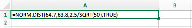
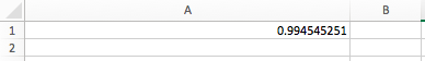
Notice that we do not get the same p-value as the graphing calculator. In this case, since it is a right-tailed test, Excel always goes from the first part of the distribution and reads left to right. We know that the distribution is 100%, so to get that upper portion of the distribution, we have to calculate 100%, or 1, minus this value.
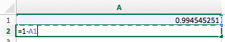
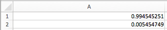
We get the same p-value, which is about 0.0054, or 0.54%.
Source: THIS TUTORIAL WAS AUTHORED BY JONATHAN OSTERS FOR SOPHIA LEARNING. PLEASE SEE OUR TERMS OF USE.