Table of Contents |
Remember, a critical value is a value that corresponds to the number of standard deviations away from the mean that we're willing to attribute to chance. How far from the center of our distribution can a t-test statistic fall? We'll decide to either fail to reject the null hypothesis or reject the null hypothesis.
For a left-tailed test, let's find the critical t* for a hypothesis test, with eight degrees of freedom, that would reject the H0 at a 2.5% significance level.
One way to do this is with a graphing calculator. However, depending on the type of calculator you have, you may or may not have this function. If you have the TI-84, the TI-89, the Nspire, or the CAS, you should have the function for doing the inverse T. If you do not have one of these calculators, you can also use Excel, which will be explained later.
First, click "2nd," "DIST," and the inverse T, or "InvT." Because we are looking at a left-tailed test, we're looking at the bottom 2.5% of the distribution. We will want to enter 0.025, and then 8 for the degrees of freedom. Remember, our distribution changes shape based on the sample size.
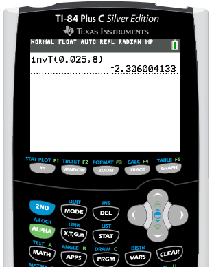
We get a corresponding critical t-value of negative 2.306. This falls about here on the distribution, where the lower shaded region corresponds to the lower 2.5% of our distribution, or negative 2.306.
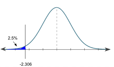
Any t-test statistic that we calculate for this corresponding hypothesis test that is less than negative 2.306 means we would reject the null hypothesis. Anything greater than that critical value is in this safe region that is unshaded. We would just attribute it to chance, and we would fail to reject the null hypothesis.
Using the t-table to find our critical t-value—remember, this is a lower-tailed test—we're going to locate the closest thing to 2.5%, or 0.025, for the one-tailed probability. We also know that we have eight degrees of freedom.
| T-Distribution Critical Values | ||||||||||||
|---|---|---|---|---|---|---|---|---|---|---|---|---|
| Tail Probability, p | ||||||||||||
| One-tail | 0.25 | 0.20 | 0.15 | 0.10 | 0.05 | 0.025 | 0.02 | 0.01 | 0.005 | 0.0025 | 0.001 | 0.0005 |
| Two-tail | 0.50 | 0.40 | 0.30 | 0.20 | 0.10 | 0.05 | 0.04 | 0.02 | 0.01 | 0.005 | 0.002 | 0.001 |
| df | ||||||||||||
| 1 | 1.000 | 1.376 | 1.963 | 3.078 | 6.314 | 12.71 | 15.89 | 31.82 | 63.66 | 127.3 | 318.3 | 636.6 |
| 2 | 0.816 | 1.080 | 1.386 | 1.886 | 2.920 | 4.303 | 4.849 | 6.965 | 9.925 | 14.09 | 22.33 | 31.60 |
| 3 | 0.765 | 0.978 | 1.250 | 1.638 | 2.353 | 3.182 | 3.482 | 4.541 | 5.841 | 7.453 | 10.21 | 12.92 |
| 4 | 0.741 | 0.941 | 1.190 | 1.533 | 2.132 | 2.776 | 2.999 | 3.747 | 4.604 | 5.598 | 7.173 | 8.610 |
| 5 | 0.727 | 0.920 | 1.156 | 1.476 | 2.015 | 2.571 | 2.757 | 3.365 | 4.032 | 4.773 | 5.893 | 6.869 |
| 6 | 0.718 | 0.906 | 1.134 | 1.440 | 1.943 | 2.447 | 2.612 | 3.143 | 3.707 | 4.317 | 5.208 | 5.959 |
| 7 | 0.711 | 0.896 | 1.119 | 1.415 | 1.895 | 2.365 | 2.517 | 2.998 | 3.499 | 4.029 | 4.785 | 5.408 |
| 8 | 0.706 | 0.889 | 1.108 | 1.397 | 1.860 | 2.306 | 2.449 | 2.896 | 3.355 | 3.833 | 4.501 | 5.041 |
| 9 | 0.703 | 0.883 | 1.100 | 1.383 | 1.833 | 2.262 | 2.398 | 2.821 | 3.250 | 3.690 | 4.297 | 4.781 |
| 10 | 0.700 | 0.879 | 1.093 | 1.372 | 1.812 | 2.228 | 2.359 | 2.764 | 3.169 | 3.581 | 4.144 | 4.587 |
A tail probability of 0.025 and eight degrees of freedom is going to correspond to a critical t-value of 2.306.
Since this is a left-tailed test, we have to recognize that it's a lower-tailed test; we're lower than the mean of the distribution. So, the critical value should actually be a negative 2.306. Always be careful of that when using the t-table.
To find a critical t-value in Excel, go under the Formulas tab. We're going to insert a function. Under the Statistical column, we're going to look for T.INV, or inverse of T. We're going to put in the corresponding significance level, 0.025, comma, degrees of freedom, which was 8. Hit Enter.


Notice how we get the same value we did on the calculator and in the table—a negative 2.306.
For this second example, we're going to look at a right-tailed test and find the critical t* for a hypothesis test with only four degrees of freedom that would reject the null hypothesis at 5% significance level.
Because it's a right-tailed test, we need to find the cutoff for our t-scores. This will be on the upper part of this distribution that corresponds to the top 5% of our distribution.
On the graphing calculator, again click "2nd," "DIST," and the inverse T, or "InvT." However, we wouldn't enter 0.05 this time. Remember, we always read a distribution from left to right, or from 0% to 100%. For our right-tailed test, we're looking at the top 5%, which actually corresponds to 100% minus 5%, or the 95th percentile. We'd actually put in 0.95, comma, our degrees of freedom, which was 4.
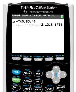
Our calculator would give us a corresponding t-test statistic of 2.132. This falls right about here on the distribution and corresponds to the top 5%.
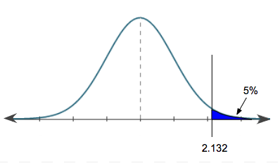
It makes sense that this is a positive value because we're above the mean. So, any t-test statistic that is above 2.132 for this particular hypothesis test means we would reject the null. Anything below that value, we'd attribute to chance, and we'd fail to reject.
Now we're going to use our t-table to find our critical t-value with a significant level of 5% for an upper-tailed test. Again, looking at our top row, which has the one-tailed probabilities, we have 5%, or 0.05. We also are looking at four degrees of freedom.
| T-Distribution Critical Values | ||||||||||||
|---|---|---|---|---|---|---|---|---|---|---|---|---|
| Tail Probability, p | ||||||||||||
| One-tail | 0.25 | 0.20 | 0.15 | 0.10 | 0.05 | 0.025 | 0.02 | 0.01 | 0.005 | 0.0025 | 0.001 | 0.0005 |
| Two-tail | 0.50 | 0.40 | 0.30 | 0.20 | 0.10 | 0.05 | 0.04 | 0.02 | 0.01 | 0.005 | 0.002 | 0.001 |
| df | ||||||||||||
| 1 | 1.000 | 1.376 | 1.963 | 3.078 | 6.314 | 12.71 | 15.89 | 31.82 | 63.66 | 127.3 | 318.3 | 636.6 |
| 2 | 0.816 | 1.080 | 1.386 | 1.886 | 2.920 | 4.303 | 4.849 | 6.965 | 9.925 | 14.09 | 22.33 | 31.60 |
| 3 | 0.765 | 0.978 | 1.250 | 1.638 | 2.353 | 3.182 | 3.482 | 4.541 | 5.841 | 7.453 | 10.21 | 12.92 |
| 4 | 0.741 | 0.941 | 1.190 | 1.533 | 2.132 | 2.776 | 2.999 | 3.747 | 4.604 | 5.598 | 7.173 | 8.610 |
| 5 | 0.727 | 0.920 | 1.156 | 1.476 | 2.015 | 2.571 | 2.757 | 3.365 | 4.032 | 4.773 | 5.893 | 6.869 |
| 6 | 0.718 | 0.906 | 1.134 | 1.440 | 1.943 | 2.447 | 2.612 | 3.143 | 3.707 | 4.317 | 5.208 | 5.959 |
| 7 | 0.711 | 0.896 | 1.119 | 1.415 | 1.895 | 2.365 | 2.517 | 2.998 | 3.499 | 4.029 | 4.785 | 5.408 |
That will correspond to a t-test statistic, or in this case, a critical t* of 2.132. Because it is an upper-tailed test, we're above the center of the distribution, so it should be positive. We're going to leave the t-test statistic as a positive 2.132.
Now let's use Excel to find our critical t-value. Again, go under our Formulas tab and look under the Statistical column for T.INV, or inverse T. In this case, remember that because it's an upper-tailed test, we have to put in 95%, or 0.95, since that corresponds to the upper 5% from a cutoff value. Next, enter a comma, and then our degrees of freedom, which was 4.


We get the same critical t-value we did in our calculator and on our table—a positive 2.132.
For this last example, we're going to look at a two-sided test and find the critical t-value for a hypothesis test with 13 degrees of freedom that would reject the null hypothesis at 1% significance level.
Because it's a two-sided test, we have to divide the significance level of 1%, or 0.01, into both sides of our distribution. Half of 0.01 is equal to 0.005. This means we're going to be finding that critical value, that cutoff, for the lower 0.5%, or 0.005, of the distribution and the upper 0.5% of our distribution.
On the graphing calculator, for the lower 0.5%, we would do "invT(0.005,13)."
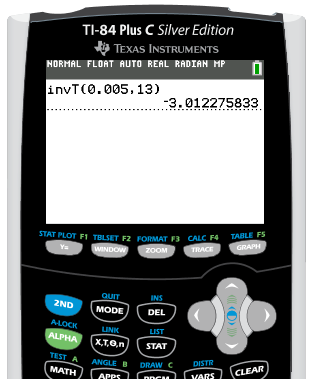
We would get a corresponding critical t-value of negative 3.012, which is about here on our distribution.
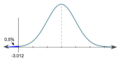
This would correspond to the lower 0.5% of our distribution, and it should be negative since it's below the mean. We're going to do the same thing, but for the upper 0.5% of our distribution. Remember, in our distribution, we always read left to right from 0% to 100%. So, upper 0.5% actually corresponds to 99.5%, or 0.995, of our distribution. On the graphing calculator, we would enter "invT(0.995,13)."
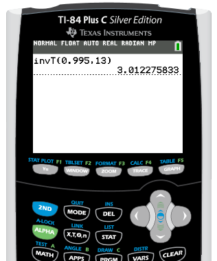
We get a positive 3.012. Our distribution now looks like this:
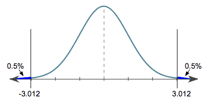
For this particular hypothesis test, if we got a t-test statistic that was above a positive 3.012 or below a negative 3.012, we would reject the null. Anything in between, we'd attribute to chance, and we would fail to reject the null.
Now we're going to use our t-table to find our critical t-value. We had 13 degrees of freedom, and our significance level was 1%. Keep in mind that this is the tail probability for two tails, meaning each tail will have 0.5%.
If you take a look at our table, we actually have both one-tailed and two-tailed probabilities listed. You can use either row and get the same critical value.
| T-Distribution Critical Values | ||||||||||||
|---|---|---|---|---|---|---|---|---|---|---|---|---|
| Tail Probability, p | ||||||||||||
| One-tail | 0.25 | 0.20 | 0.15 | 0.10 | 0.05 | 0.025 | 0.02 | 0.01 | 0.005 | 0.0025 | 0.001 | 0.0005 |
| Two-tail | 0.50 | 0.40 | 0.30 | 0.20 | 0.10 | 0.05 | 0.04 | 0.02 | 0.01 | 0.005 | 0.002 | 0.001 |
| df | ||||||||||||
| 1 | 1.000 | 1.376 | 1.963 | 3.078 | 6.314 | 12.71 | 15.89 | 31.82 | 63.66 | 127.3 | 318.3 | 636.6 |
| 2 | 0.816 | 1.080 | 1.386 | 1.886 | 2.920 | 4.303 | 4.849 | 6.965 | 9.925 | 14.09 | 22.33 | 31.60 |
| 3 | 0.765 | 0.978 | 1.250 | 1.638 | 2.353 | 3.182 | 3.482 | 4.541 | 5.841 | 7.453 | 10.21 | 12.92 |
| 4 | 0.741 | 0.941 | 1.190 | 1.533 | 2.132 | 2.776 | 2.999 | 3.747 | 4.604 | 5.598 | 7.173 | 8.610 |
| 5 | 0.727 | 0.920 | 1.156 | 1.476 | 2.015 | 2.571 | 2.757 | 3.365 | 4.032 | 4.773 | 5.893 | 6.869 |
| 6 | 0.718 | 0.906 | 1.134 | 1.440 | 1.943 | 2.447 | 2.612 | 3.143 | 3.707 | 4.317 | 5.208 | 5.959 |
| 7 | 0.711 | 0.896 | 1.119 | 1.415 | 1.895 | 2.365 | 2.517 | 2.998 | 3.499 | 4.029 | 4.785 | 5.408 |
| 8 | 0.706 | 0.889 | 1.108 | 1.397 | 1.860 | 2.306 | 2.449 | 2.896 | 3.355 | 3.833 | 4.501 | 5.041 |
| 9 | 0.703 | 0.883 | 1.100 | 1.383 | 1.833 | 2.262 | 2.398 | 2.821 | 3.250 | 3.690 | 4.297 | 4.781 |
| 10 | 0.700 | 0.879 | 1.093 | 1.372 | 1.812 | 2.228 | 2.359 | 2.764 | 3.169 | 3.581 | 4.144 | 4.587 |
| 11 | 0.697 | 0.876 | 1.088 | 1.363 | 1.796 | 2.201 | 2.328 | 2.718 | 3.106 | 3.497 | 4.025 | 4.437 |
| 12 | 0.695 | 0.873 | 1.083 | 1.356 | 1.782 | 2.179 | 2.303 | 2.681 | 3.055 | 3.428 | 3.930 | 4.318 |
| 13 | 0.694 | 0.870 | 1.079 | 1.350 | 1.771 | 2.160 | 2.282 | 2.650 | 3.012 | 3.372 | 3.852 | 4.221 |
| 14 | 0.692 | 0.868 | 1.076 | 1.345 | 1.761 | 2.145 | 2.264 | 2.624 | 2.977 | 3.326 | 3.787 | 4.140 |
| 15 | 0.691 | 0.866 | 1.074 | 1.341 | 1.753 | 2.131 | 2.249 | 2.602 | 2.947 | 3.286 | 3.733 | 4.073 |
We get a corresponding critical t-value of 3.012. But because it's a two-sided test, it's both the positive and the negative 3.012.
Now we're going to use Excel to find our critical t-value for our two-sided test. This one's going to be a little bit different than the previous two, which were one-tailed tests. Again, go under the Statistical column. In this case, we're going to do the inverse of T for 2T, which means the two-tailed test.


In this case, we do not have to divide our significance level into the two halves; we can just put 0.01. Excel knows—because we indicated it's a two-tailed test—to automatically divide that 1%. We were also at 13 degrees of freedom. Therefore, it gives us the positive corresponding critical t-value of 3.012. However, we know that it's not only a positive 3.012, but also a negative 3.012.
Source: THIS TUTORIAL WAS AUTHORED BY RACHEL ORR-DEPNER FOR SOPHIA LEARNING. PLEASE SEE OUR TERMS OF USE.