Use Sophia to knock out your gen-ed requirements quickly and affordably. Learn more
×

Graphs of Polynomial Functions

Author: Sophia

what's covered
In this lesson, you will pull together all the characteristics of polynomial functions and analyze their graphs. Specifically, this lesson will cover:
  1. Determining the End Behavior of Polynomial Functions
  2. Graphs of Polynomial Functions

1. Determining the End Behavior of Polynomial Functions

Earlier in the course, we analyzed the end behavior of power functions. It turns out that the end behavior of polynomial functions is closely related to that of a power function.

Consider a polynomial function f open parentheses x close parentheses equals a subscript n x to the power of n plus a subscript n minus 1 end subscript x to the power of n minus 1 end exponent plus horizontal ellipsis plus a subscript 0, where a subscript 0 comma space a subscript 1 comma space horizontal ellipsis comma space a subscript n are real numbers. For extremely large values of x, the leading term will dominate the value of the output since the input is raised to the largest power.

The same can be said for extremely small values of x (-100, -1000, etc.).

Thus, the end behavior of a polynomial function is the same as the end behavior of its leading term.

big idea
The end behavior of a polynomial function f open parentheses x close parentheses equals a subscript n x to the power of n plus a subscript n minus 1 end subscript x to the power of n minus 1 end exponent plus horizontal ellipsis plus a subscript 0 is the same as the end behavior of g open parentheses x close parentheses equals a subscript n x to the power of n.

The end behavior of polynomial functions can be summarized using the table.

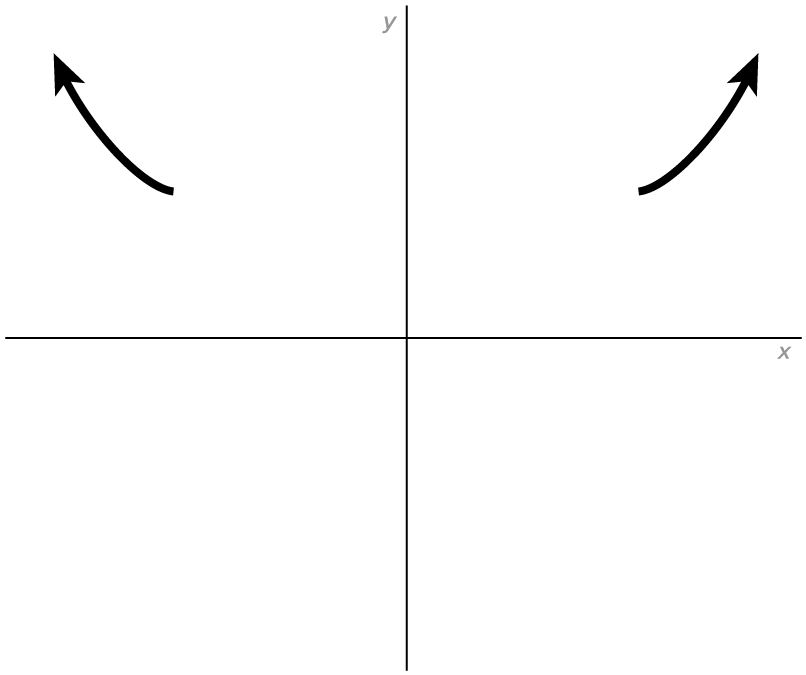
Remember that the end behavior of a power function depends on its degree (even or odd) as well as its coefficient (positive or negative).

Since the leading term of the polynomial is used to determine its end behavior, the leading coefficient of the polynomial and the degree of the polynomial are used to determine end behavior.

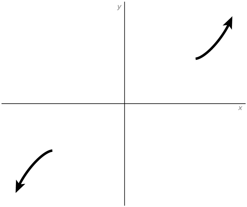
Positive Leading Coefficient, bold italic a subscript bold n bold greater than bold 0 
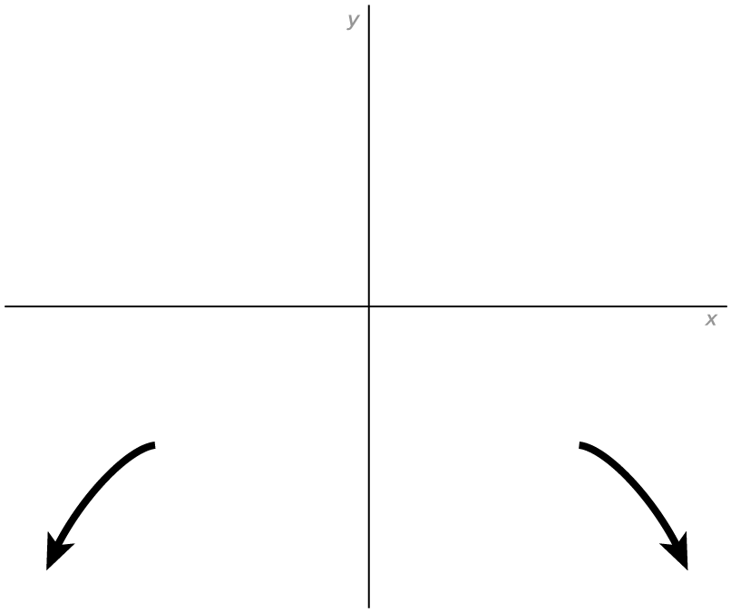
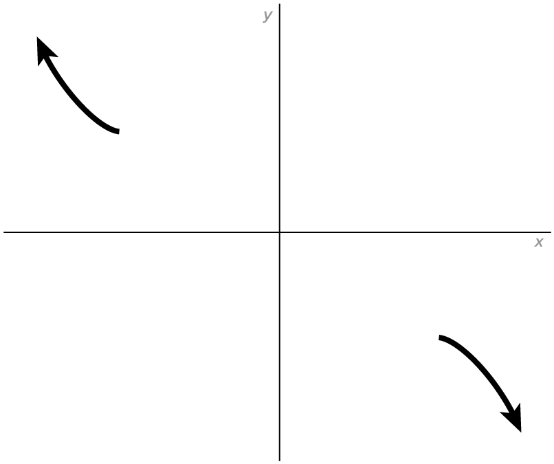
Negative Leading Coefficient, bold italic a subscript bold n bold less than bold 0
Even Degree
x rightwards arrow short dash infinity comma space f open parentheses x close parentheses rightwards arrow infinity
x rightwards arrow infinity comma space f open parentheses x close parentheses rightwards arrow infinity

x rightwards arrow short dash infinity comma space f open parentheses x close parentheses rightwards arrow short dash infinity
x rightwards arrow infinity comma space f open parentheses x close parentheses rightwards arrow short dash infinity
Odd Degree
x rightwards arrow short dash infinity comma space f open parentheses x close parentheses rightwards arrow short dash infinity
x rightwards arrow infinity comma space f open parentheses x close parentheses rightwards arrow infinity

x rightwards arrow short dash infinity comma space f open parentheses x close parentheses rightwards arrow infinity
x rightwards arrow infinity comma space f open parentheses x close parentheses rightwards arrow short dash infinity

Now that we have a process, here is an example:

EXAMPLE

Determine the end behavior of f open parentheses x close parentheses equals short dash 2 x to the power of 4 plus 5 x cubed minus 10 x squared plus 200 x plus 90.

The end behavior of f open parentheses x close parentheses is the same as the end behavior of g open parentheses x close parentheses equals short dash 2 x to the power of 4. Since the leading coefficient is negative and the degree is even, the graph falls indefinitely on both sides.

This means that as x rightwards arrow short dash infinity comma f open parentheses x close parentheses rightwards arrow short dash infinity, and as x rightwards arrow infinity comma f open parentheses x close parentheses rightwards arrow short dash infinity.

You can verify this by graphing the polynomial function.

try it
Consider the function f open parentheses x close parentheses equals x to the power of 5 minus 140 x cubed plus 20 x.


2. Graphs of Polynomial Functions

To graph a polynomial function, there are several things to consider.

The degree of the polynomial is used to determine the end behavior, possible number of x-intercepts, and possible number of turning points.

The leading coefficient, along with the degree, is used to determine the end behavior of the graph of the polynomial.

When the zeros are real, they correspond to x-intercepts. The multiplicity of the zeros of the polynomial also determines the graph’s behavior around the corresponding x-intercepts, as we will investigate now.

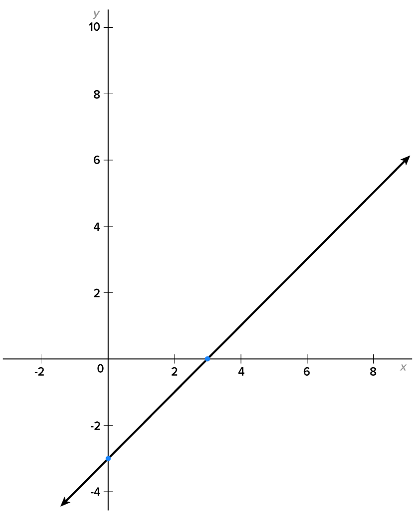
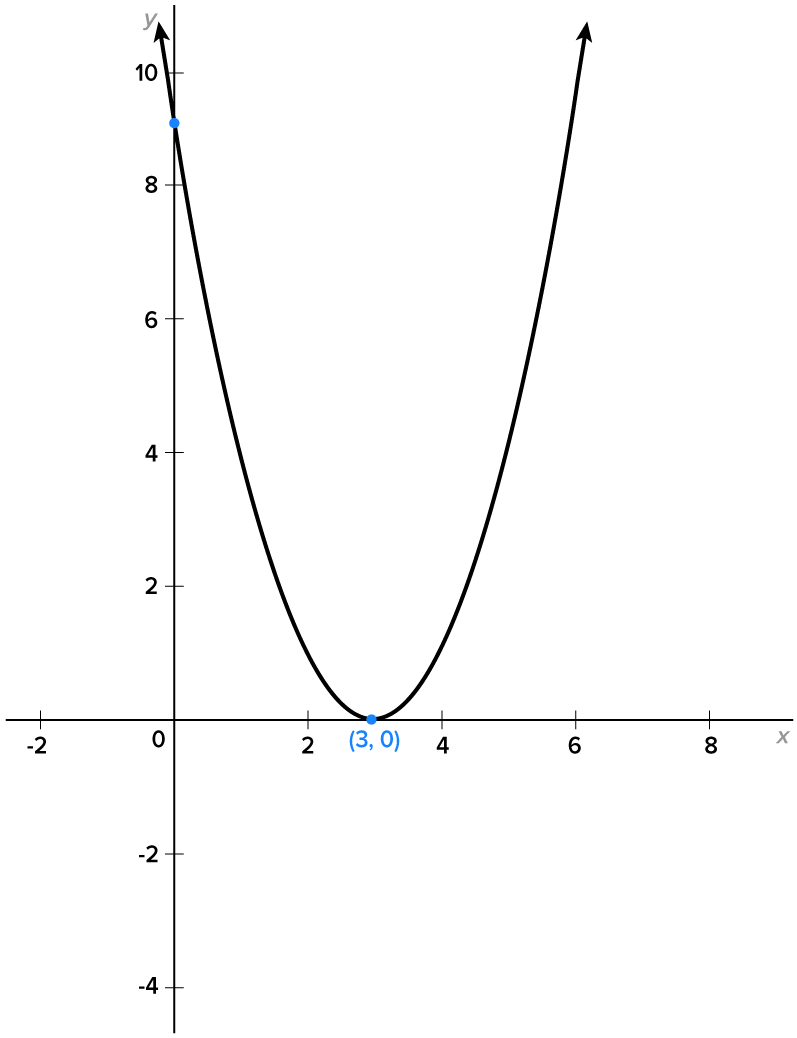
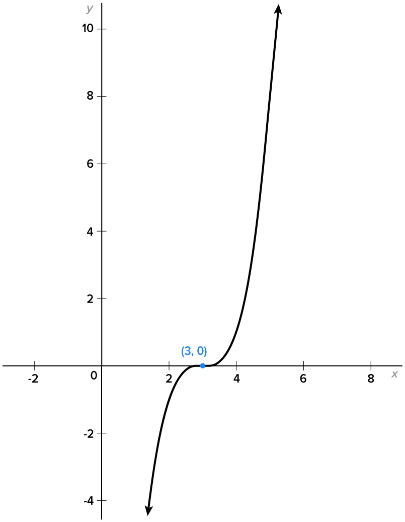
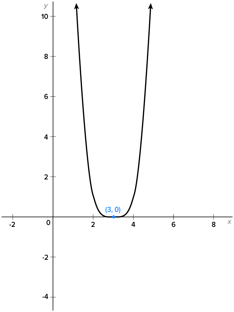
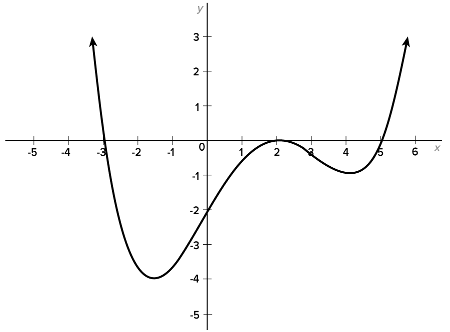
Consider the graphs below, which all have x-intercepts at open parentheses 3 comma space 0 close parentheses.

bold italic f open parentheses bold x close parentheses bold equals bold italic x bold minus bold 3 bold italic g open parentheses bold x close parentheses bold equals open parentheses bold x bold minus bold 3 close parentheses to the power of bold 2
bold italic h open parentheses bold x close parentheses bold equals open parentheses bold x bold minus bold 3 close parentheses to the power of bold 3 bold italic j open parentheses bold x close parentheses bold equals open parentheses bold x bold minus bold 3 close parentheses to the power of bold 4

Note the behavior of the graph around the x-intercept open parentheses 3 comma space 0 close parentheses.

In the graphs of f open parentheses x close parentheses equals x minus 3 and h open parentheses x close parentheses equals open parentheses x minus 3 close parentheses cubed comma the graph crosses the axis at open parentheses 3 comma space 0 close parentheses. Also notice in the graph of h open parentheses x close parentheses equals open parentheses x minus 3 close parentheses cubed that the graph “levels out” at the x-intercept before crossing the axis.

In the graphs of g open parentheses x close parentheses equals open parentheses x minus 3 close parentheses squared and j open parentheses x close parentheses equals open parentheses x minus 3 close parentheses to the power of 4 comma the graph touches the axis at open parentheses 3 comma space 0 close parentheses. Also notice in the graph of j open parentheses x close parentheses equals open parentheses x minus 3 close parentheses to the power of 4 is flatter around its x-intercept at left parenthesis 3 comma 0 right parenthesis.

Based on this, we can make the following generalization.

big idea
If a is a real number, and if open parentheses x minus a close parentheses to the power of k is a factor of a polynomial function f open parentheses x close parentheses comma then the graph crosses the x-axis at open parentheses a comma space 0 close parentheses if k is odd, and touches the axis at open parentheses a comma space 0 close parentheses when k is even.

Now that we have all the pieces, we can analyze polynomial functions and sketch their graphs.

EXAMPLE

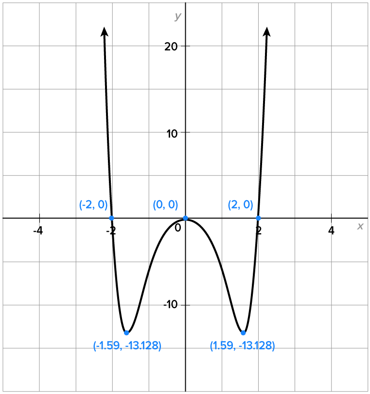
Find all relevant characteristics of the graph of f open parentheses x close parentheses equals x to the power of 6 minus 3 x to the power of 4 minus 4 x squared.

Note that the degree is 6 and the leading coefficient is positive. This means that the graph rises indefinitely to the left and right. In other words, as x rightwards arrow short dash infinity comma f open parentheses x close parentheses rightwards arrow infinity, and as x rightwards arrow infinity comma f open parentheses x close parentheses rightwards arrow infinity.

Since the degree is 6, the graph can have at most six x-intercepts and at most five turning points.

First, factor the polynomial:

table attributes columnalign left end attributes row cell f open parentheses x close parentheses equals x to the power of 6 minus 3 x to the power of 4 minus 4 x squared end cell row cell f open parentheses x close parentheses equals x squared open parentheses x to the power of 4 minus 3 x squared minus 4 close parentheses end cell row cell f open parentheses x close parentheses equals x squared open parentheses x squared minus 4 close parentheses open parentheses x squared plus 1 close parentheses end cell row cell f open parentheses x close parentheses equals x squared open parentheses x plus 2 close parentheses open parentheses x minus 2 close parentheses open parentheses x squared plus 1 close parentheses end cell end table

By inspection, the zeros of f open parentheses x close parentheses are 0 (with multiplicity 2), -2, 2, and plus-or-minus i.

Note: the zeros plus-or-minus i do not correspond to x-intercepts since they are imaginary.

This means that the graph crosses the x-axis at open parentheses short dash 2 comma space 0 close parentheses and open parentheses 2 comma space 0 close parentheses comma and touches the x-axis at open parentheses 0 comma space 0 close parentheses. Since one of the x-intercepts is at open parentheses 0 comma space 0 close parentheses comma we also already have the y-intercept.

The graph of f open parentheses x close parentheses is shown below.


Note that all the characteristics we found from the equation are present. All of the key points (intercepts and turning points) are labeled.

Note: the graph has three x-intercepts and three turning points.

Before looking at a different type of problem, here is something to consider.

think about it
Does multiplying a polynomial function by a constant affect the zeros of the function? Consider the functions f open parentheses x close parentheses equals open parentheses x plus 5 close parentheses squared open parentheses x minus 3 close parentheses and g open parentheses x close parentheses equals short dash 4 open parentheses x plus 5 close parentheses squared open parentheses x minus 3 close parentheses.

Hopefully, you found that the zeros of each function are the same, therefore the “-4” has no effect on the zeros. In general, y equals f open parentheses x close parentheses and y equals a times f open parentheses x close parentheses have the same zeros. This information is helpful in writing a possible equation for a given polynomial graph. When doing so, the smallest possible degree is desired.

EXAMPLE

Write a possible equation with smallest degree for the polynomial that has the graph shown below.


Here is what to consider to write the best equation for this graph.

End behavior: the graph falls to the left and rises to the right. This means that the polynomial has an odd degree and a positive leading coefficient.

Intercepts/zeros: there are three x-intercepts, and the graph crosses the x-axis at each x-intercept. Since the graph crosses and doesn’t flatten out at these x-intercepts, and since we also want the polynomial with smallest degree, this suggests that each zero (-2, 1, and 3) has multiplicity 1. Therefore, f open parentheses x close parentheses 
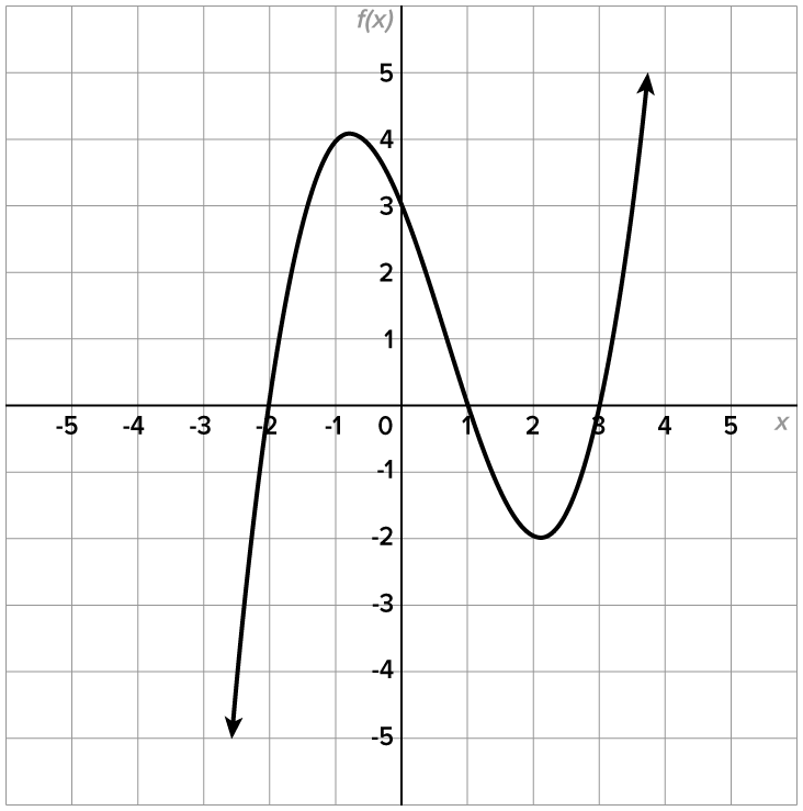
has a degree of at least 3.

Turning points: there are two turning points, which suggests that the degree is at least 3.

y-intercept: the y-intercept is located at open parentheses 0 comma space 3 close parentheses.

To write the equation, remember that each zero corresponds to a factor of f open parentheses x close parentheses. Also remember that any constant multiple, a comma can be placed in front of the expression, which doesn’t affect the zeros.

  • The zero x equals short dash 2 corresponds to the factor open parentheses x plus 2 close parentheses.
  • The zero x equals 1 corresponds to the factor open parentheses x minus 1 close parentheses.
  • The zero x equals 3 corresponds to the factor open parentheses x minus 3 close parentheses.
This means that a possible equation for this function is f open parentheses x close parentheses equals a open parentheses x plus 2 close parentheses open parentheses x minus 1 close parentheses open parentheses x minus 3 close parentheses.

Note that this equation is built from the zeros. We also need to consider the y-intercept.

Since (0, 3) is the y-intercept of the graph, we know that f open parentheses 0 close parentheses equals 3.

According to the function we built, f open parentheses 0 close parentheses equals a open parentheses 2 close parentheses open parentheses short dash 1 close parentheses open parentheses short dash 3 close parentheses equals 6 a.

Thus, 6 a equals 3 comma which means a equals 1 half.

Finally, a possible equation for this graph is f open parentheses x close parentheses equals 1 half open parentheses x plus 2 close parentheses open parentheses x minus 1 close parentheses open parentheses x minus 3 close parentheses.

In expanded form, f open parentheses x close parentheses equals 1 half x cubed minus x squared minus 5 over 2 x plus 3.

Here is another example in which multiplicity is considered:

EXAMPLE

Write a possible equation for the polynomial graph shown below.
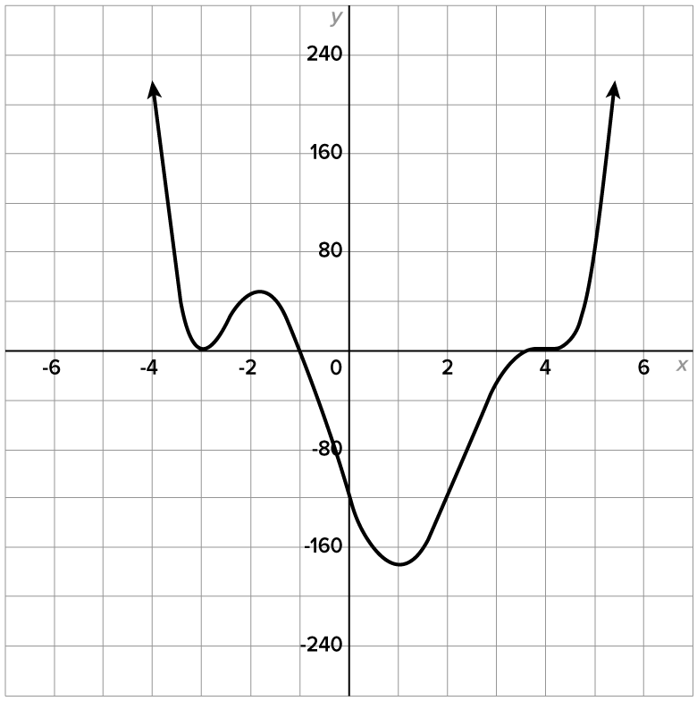


Here is what to consider to write the best equation for this graph:

End behavior: the graph rises to the left and rises to the right. This means that the polynomial has an even degree and a positive leading coefficient.

Intercepts/zeros: there are three x-intercepts: open parentheses short dash 3 comma space 0 close parentheses comma open parentheses short dash 1 comma space 0 close parentheses comma and open parentheses 4 comma space 0 close parentheses.

  • The graph touches the x-axis at open parentheses short dash 3 comma space 0 close parentheses comma suggesting that -3 is a zero with multiplicity 2.
  • The graph crosses the x-axis at open parentheses short dash 1 comma space 0 close parentheses comma suggesting that -1 is a zero with multiplicity 1.
  • The graph crosses the x-axis at open parentheses 4 comma space 0 close parentheses comma but the curve flattens out around the intercept. This suggests that 4 is a zero with multiplicity 3.
Turning points: there are three turning points, which suggests that the degree is at least 4.

y-intercept: the y-intercept is located at open parentheses 0 comma space short dash 120 close parentheses.

To write the equation, remember that each zero corresponds to a factor of f open parentheses x close parentheses. Also remember that any constant multiple can be placed in front of the expression, which doesn’t affect the zeros.

  • The zero x equals short dash 3 with multiplicity 2 corresponds to the factor open parentheses x plus 3 close parentheses squared.
  • The zero x equals short dash 1 corresponds to the factor open parentheses x plus 1 close parentheses.
  • The zero x equals 4 with multiplicity 3 corresponds to the factor open parentheses x minus 4 close parentheses cubed.
This means that a possible equation for this function is f open parentheses x close parentheses equals a open parentheses x plus 3 close parentheses squared open parentheses x plus 1 close parentheses open parentheses x minus 4 close parentheses cubed.

Note that this equation is built from the zeros. We also need to consider the y-intercept.

Since open parentheses 0 comma space short dash 120 close parentheses is the y-intercept of the graph, we know that f open parentheses 0 close parentheses equals short dash 120.

According to the function we built, f open parentheses 0 close parentheses equals a open parentheses 3 close parentheses squared open parentheses 1 close parentheses open parentheses short dash 4 close parentheses cubed equals short dash 576 a. Then, short dash 576 a equals short dash 120 comma which means a equals 5 over 24.

Finally, a possible equation for this graph is f open parentheses x close parentheses equals 5 over 24 open parentheses x plus 3 close parentheses squared open parentheses x plus 1 close parentheses open parentheses x minus 4 close parentheses cubed. This means f open parentheses x close parentheses is a polynomial function with degree 6.

In expanded form, f open parentheses x close parentheses equals 5 over 24 x to the power of 6 minus 25 over 24 x to the power of 5 minus 35 over 8 x to the power of 4 plus 505 over 24 x cubed plus 205 over 6 x squared minus 110 x minus 120.

Notice that in the previous example, the resulting polynomial has degree 6, and the sum of the multiplicities is 2 plus 1 plus 3 equals 6. This is not a coincidence.

big idea
The sum of the multiplicities of the zeros of a polynomial function is equal to the degree of the polynomial function.

summary
In this lesson, you learned that the end behavior of a polynomial function is the same as the end behavior of its leading term; therefore, the leading coefficient of the polynomial and the degree of the polynomial are used to determine the end behavior of the polynomial function. You also learned that there are many characteristics of an equation that are connected with the graph of a polynomial function. Assuming the zero is real, each factor of a polynomial function corresponds to a zero, which in turn corresponds to an x-intercept of the graph. The degree of the polynomial, along with the sign of the leading coefficient, determines the end behavior of the graph of the polynomial. The multiplicity of each zero determines whether or not the graph of the polynomial crosses or touches the x-axis. Lastly, the sum of the multiplicities of each zero is equal to the degree of the polynomial.
SOURCE: THIS WORK IS ADAPTED FROM PRECALCULUS BY JAY ABRAMSON. ACCESS FOR FREE AT OPENSTAX.ORG/BOOKS/PRECALCULUS/PAGES/1-INTRODUCTION-TO-FUNCTIONS