Table of Contents |
Consider the function  A table of values as well as its graph are shown below.

|

|
|---|---|
| -3 |

|
| -2 |

|
| -1 |

|
| 0 |

|
| 1 |

|
| 2 |

|
| 3 |

|
| 4 |

|
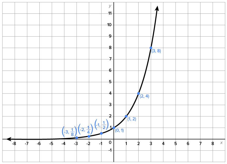

 from above, and as

 has a horizontal asymptote of
 and the range is
 is
is  Its table of values and graph are shown below.
|
|

|
|---|---|
|
|
-3 |
|
|
-2 |
|
|
-1 |
|
|
0 |
|
|
1 |
|
|
2 |
|
|
3 |
|
|
4 |
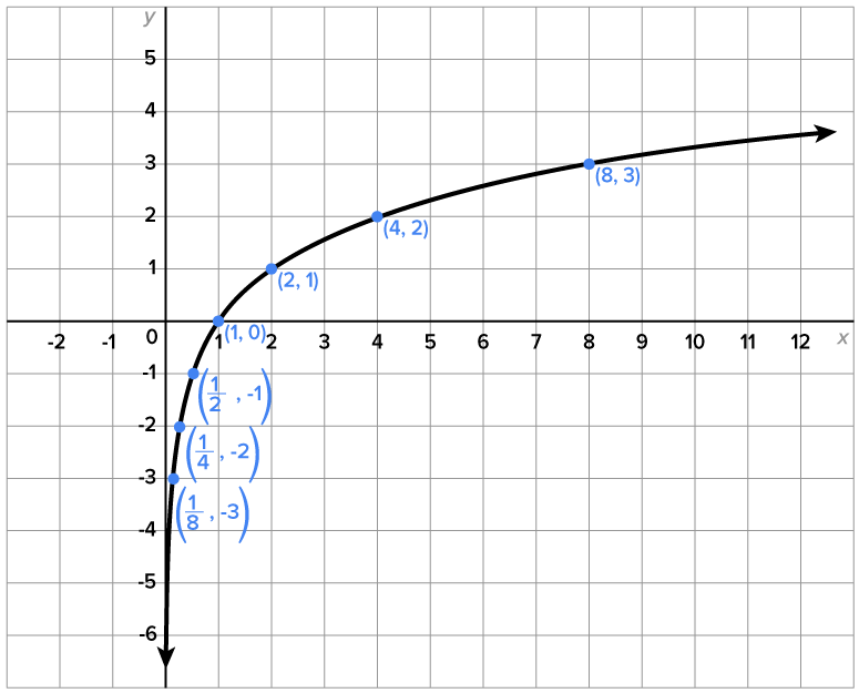
 from the right,
  , and as
 has a vertical asymptote of
 and the range is
 the graph of
  has a shape similar to the graph of This means that the graph of
  when will look similar to the graph of This includes
  since e is approximately 2.71828, which is greater than 1, and
  which is base 10.
 and
and  the graph of
  passes through the point
  Then, the graph of its inverse,
  , passes through the point
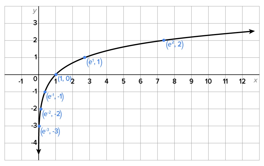
EXAMPLE
Sketch the graph of
|
|

|

|

|
1 |

|

|

|
|---|---|---|---|---|---|---|---|
|
Approximate
|
0.0498 | 0.1353 | 0.3679 | 1 | 2.7183 | 7.3891 | 20.0855 |

|
-3 | -2 | -1 | 0 | 1 | 2 | 3 |
Note the vertical asymptote
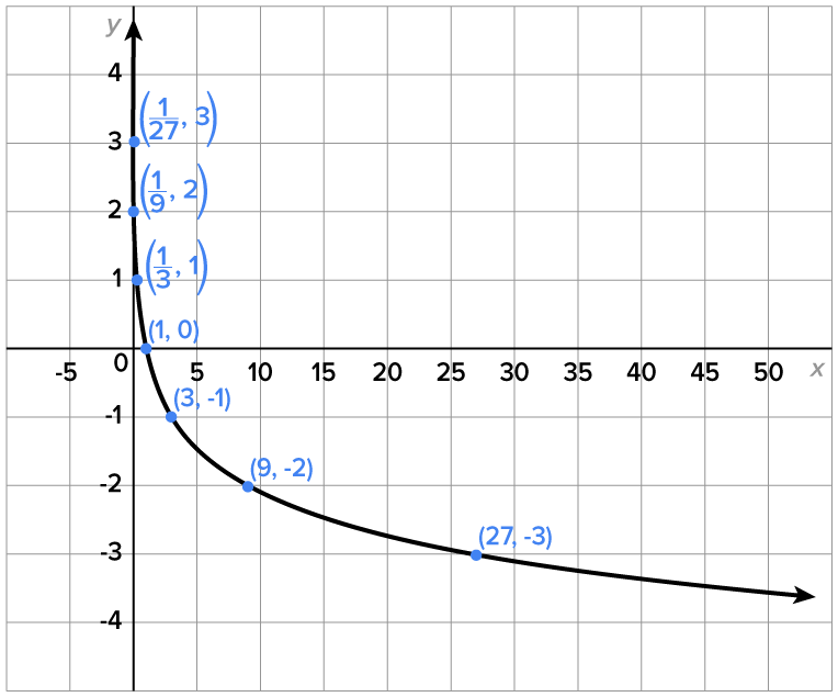
Consider the function  A table of values as well as its graph are shown below.
|
|

|
|---|---|
| -3 | 27 |
| -2 | 9 |
| -1 | 3 |
| 0 | 1 |
| 1 |

|
| 2 |

|
| 3 |

|
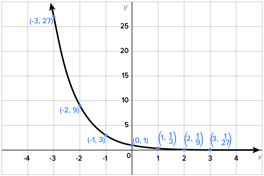
 , and as from above.
 has a horizontal asymptote of and the range is
is
has a horizontal asymptote of and the range is
is  Its table of values and graph are shown below.
|
|

|
|---|---|
|
|
3 |
|
|
2 |
|
|
1 |
| 1 | 0 |
| 3 | -1 |
| 9 | -2 |
| 27 | -3 |
from the right,  , and as
 has a vertical asymptote of and the range is
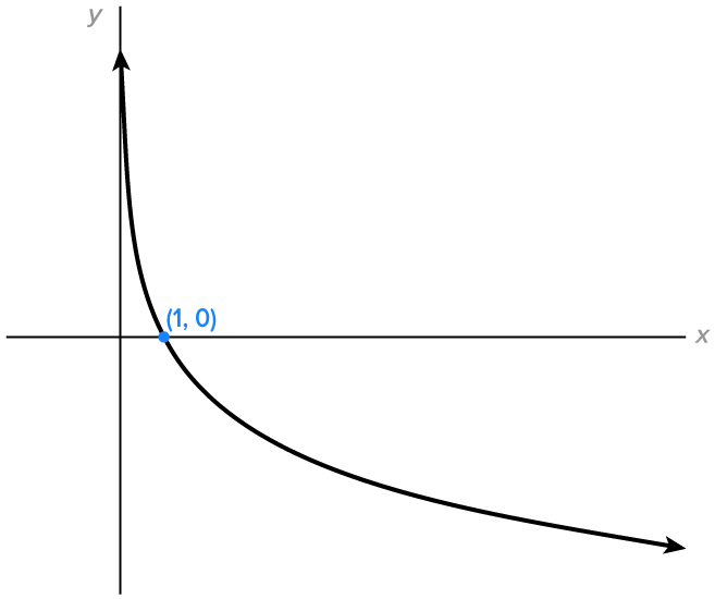
 the graph of has a shape similar to the graph of This means that the graph of when will look similar to the graph of
 and the graph of passes through the points
  and
and  Then, the graph of its inverse, , passes through the points
  and
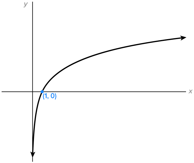
and  This means that
  and
and  for all values of b such that and
In summary, here are the possible shapes of 

|

|
|---|---|
|
|
and the domain of  is and its range is Also note the following:
the function is decreasing on its domain. the function is increasing on its domain.
is and its range is Also note the following:
the function is decreasing on its domain. the function is increasing on its domain.Since the graph of a logarithmic function passes the horizontal line test, logarithmic functions are also one-to-one. Then, logarithmic functions also have the inverse property.
The one-to-one property for logarithmic functions tells us that if two logarithmic expressions with the same base are equal to each other, then the arguments must also be equal. It also tells us that if two quantities are equal, their logarithms in the same base are also equal. This property will be used more frequently when solving equations.
 where and Then, for quantities R and S,
  if and only if
Now that we know what the graph of a logarithmic function looks like, we can observe relationships between different graphs.
First, let’s compare two logarithmic graphs with different bases.
EXAMPLE
In this example, we’ll graph and
and  on the same pair of axes.
|
|
|
|
|
1 | 2 | 4 | 8 |
|---|---|---|---|---|---|---|---|

|
-3 | -2 | -1 | 0 | 1 | 2 | 3 |
|
|

|

|

|
1 | 5 | 25 | 125 |
|---|---|---|---|---|---|---|---|

|
-3 | -2 | -1 | 0 | 1 | 2 | 3 |
and the thicker graph is 
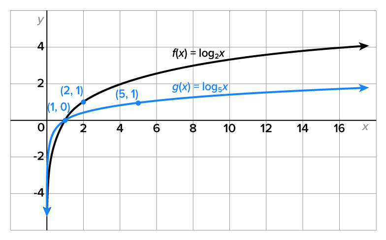 and have vertical asymptote
 the graph of g is above the graph of f.
  the graph of f is above the graph of g. the logarithmic function with the smaller base will be above the graph of the logarithmic function with the larger base. Later in this course, we will actually see that the graphs of f and g are constant multiples of one another.
 and the other is
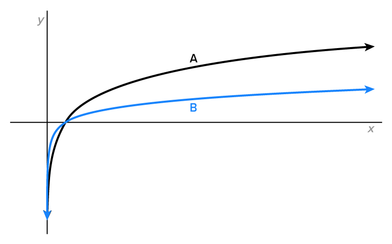
 and Graph B is
Let’s now do an exploration where we compare two logarithmic functions, but this time, the bases are reciprocals of each other.
EXAMPLE
Consider the functions and The table below shows their values for selected values of x.
|
|
|
|
|
1 | 3 | 9 | 27 |
|---|---|---|---|---|---|---|---|

|
-3 | -2 | -1 | 0 | 1 | 2 | 3 |
|
|
3 | 2 | 1 | 0 | -1 | -2 | -3 |
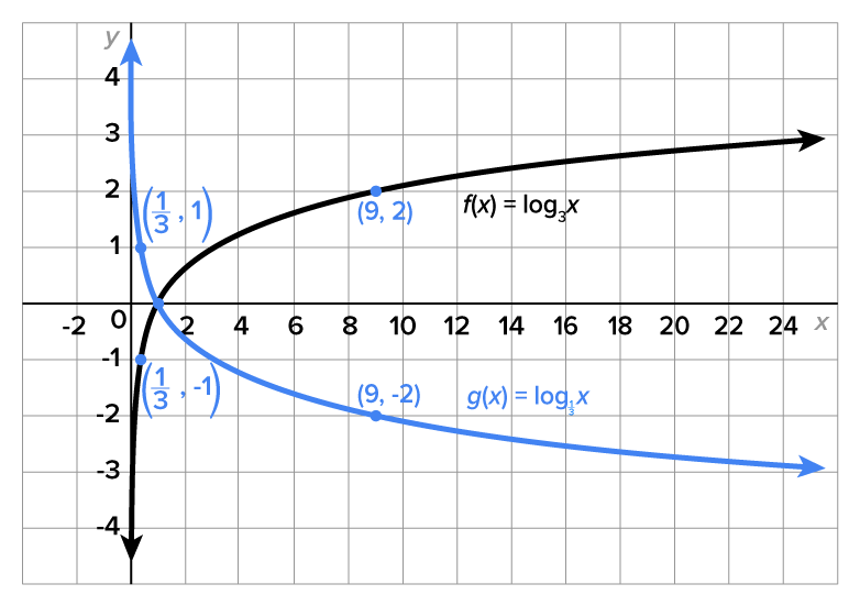

As a result of the last example, we have the following.

This result is important since it establishes a correspondence between logarithms with bases that are reciprocals of each other. Going forward, you’ll notice that all applications seen in this course (and in future courses) use bases that are larger than 1. This is because the common and natural logarithms both use bases that are larger than 1.
 and
and  are reflections of each other over the x-axis. Because of this fact, we focus on logarithmic functions with bases that are greater than 1. This way, we can still reference the natural and common logarithms.
SOURCE: THIS TUTORIAL HAS BEEN ADAPTED FROM OPENSTAX "PRECALCULUS” BY JAY ABRAMSON. ACCESS FOR FREE AT OPENSTAX.ORG/DETAILS/BOOKS/PRECALCULUS-2E. LICENSE: CREATIVE COMMONS ATTRIBUTION 4.0 INTERNATIONAL.
Consider the function  where
where  and
and  Then, for quantities R and S,
  if and only if
For any base 

 and
and 
 so
so 