Use Sophia to knock out your gen-ed requirements quickly and affordably. Learn more
×

Formatting Data

Author: Sophia

what's covered

1. Description of Netflix Data

The concepts for preparing and cleaning data for the next several tutorials will be illustrated with Netflix data from Kaggle. The full Netflix dataset is available on Kaggle and contains a comprehensive collection of information about movies and TV shows available on Netflix. For this course's purposes, we modified the data set to give you a more focused and manageable learning experience.


2. Formatting Data in Excel

Formatting in Excel is the process of changing the appearance of your data. Formatting allows you to enhance readability by making it easier for users to interpret and understand the information. When data is formatted and standardized (one of the data cleaning steps), users of the data can better determine what the data on the spreadsheet is “saying”. Consistent data formats, decimal places, and alignment prevent errors during analysis. Conditional formatting allows you to emphasize specific values or patterns. For example, you can highlight cells with the highest or lowest values, identify duplicates, or color-code data based on specific criteria.

In the following sections, you will format data values related to a Netflix data set.

2a. Formatting Numbers

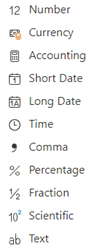
Excel offers a variety of formatting tools to help users present numerical data clearly and effectively, depending on the type of analysis you are performing and the visualization(s) you want to show. Some of the most commonly used formatting options are illustrated below.

The list of formatting options includes: Number, Currency, Accounting, Short Date, Long Date, Time, Comma, Percentage, Fraction, Scientific, and Text.

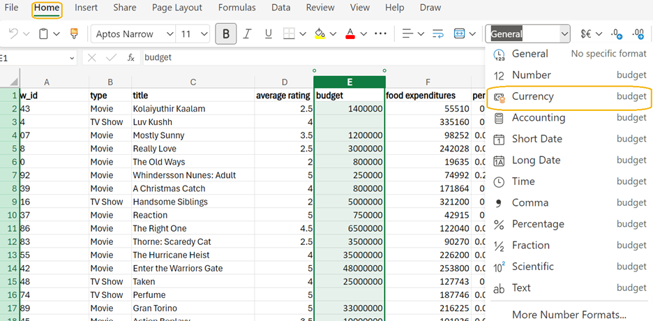
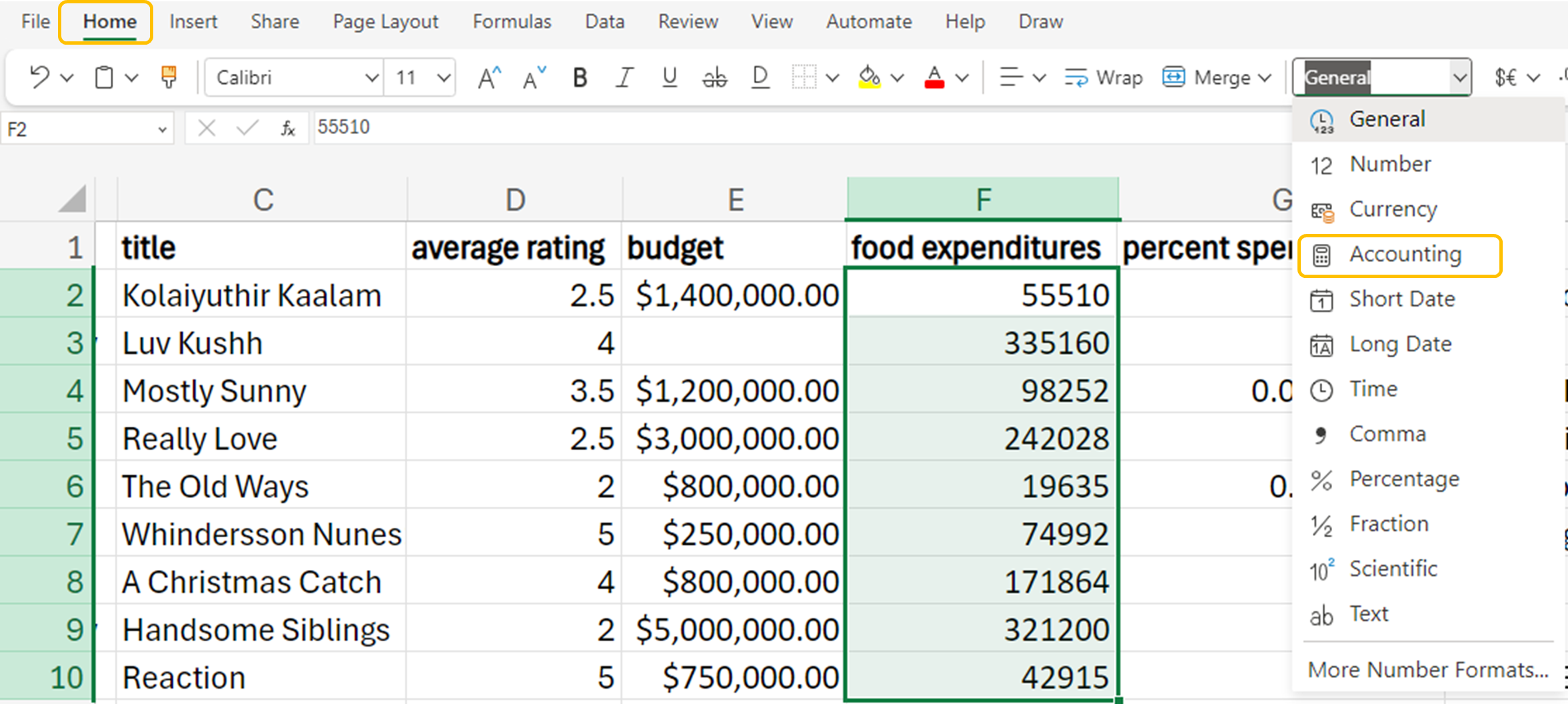
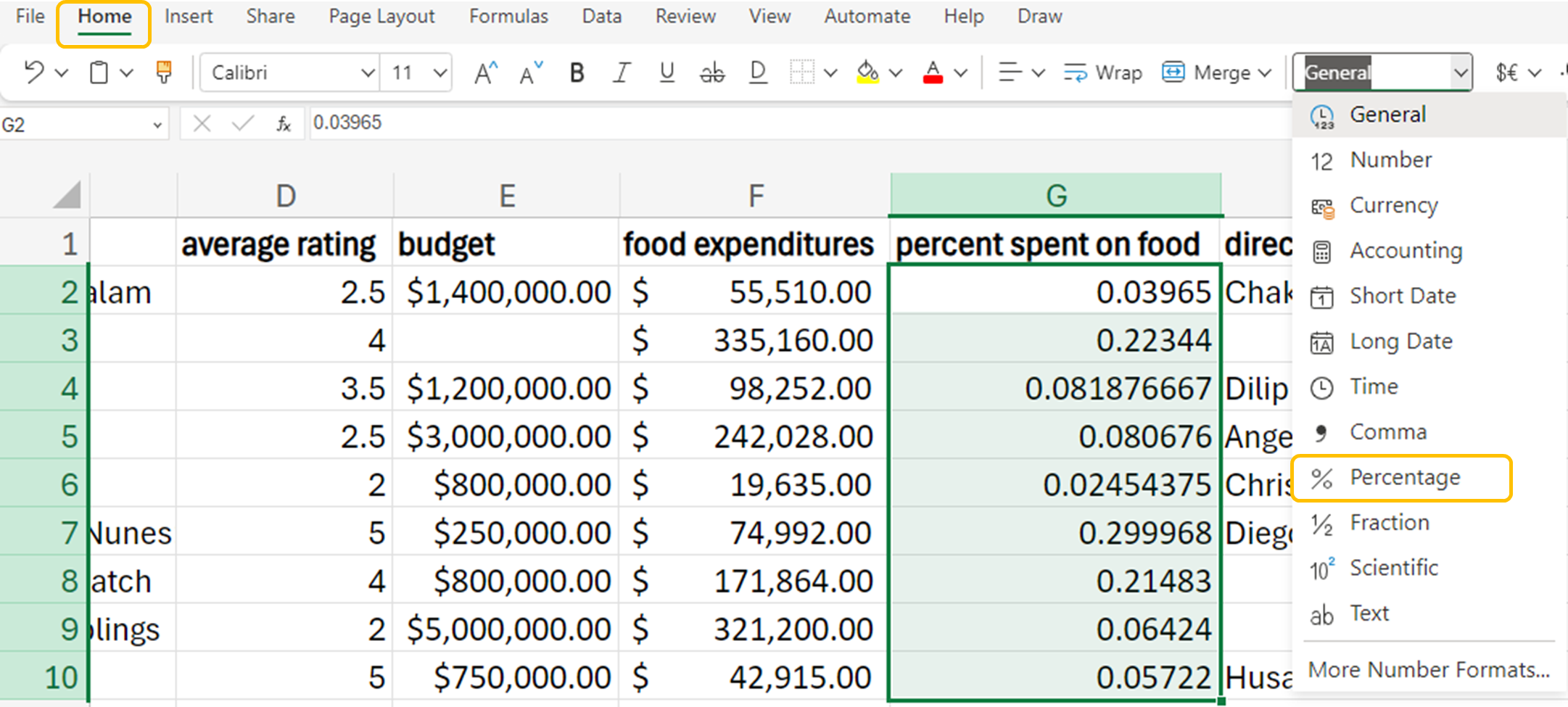
Screenshot locating the format menu

General
The General format is the default number format that Excel applies when you enter a number. It displays numbers as they are typed, without any specific formatting. For example, if you enter 1234.567, it will appear exactly as 1234.567.

Since general formatting is the default format in Excel and because this dataset has yet to be cleaned, all of the columns in Netflix.xlsx have general formatting applied, except for date_added.

Currency
The Currency format is used for monetary values and displays the currency symbol next to the number. It also allows for the specification of decimal places. For example, if you format 1234.567 as currency with two decimal places, it will appear as $1,234.57.

EXAMPLE

Currency formatting applies dollar signs ($) and decimal places to the budget column.
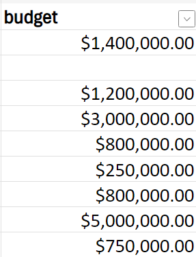
Data on the left shows unformatted numbers and on the right shows the same numbers formatted as currency with dollar signs and two decimal places. 

try it
Format the budget column in currency formatting (adding a dollar sign and two decimal places).

  1. Open netflix.xlsx.
  2. Select the budget column.
  3. On the ribbon home menu select the drop-down arrow in the Number Format tool from the Home menu. Select Currency.


    You should then see the budget column update to the desired format.
  4. Check your work by comparing your formatted budget column to the one in the example.

Comma
Alternatively, the comma format is used to display numbers with the thousand's place separators (,) and a specified number of decimal places. For example, 1234.567 formatted with the comma style and two decimal places would appear as 1,234.57. Comparing this to the currency, the comma and decimal places appear, but the $ is no longer included.

EXAMPLE

In Excel, you can apply a comma format. Comma formatting applies a thousands separator and two decimal places to the budget column.
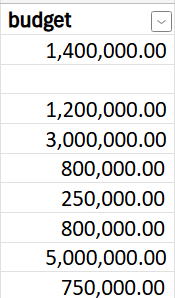
try it
Format the budget column using comma formatting by adding a thousands separator and two decimal places.

  1. Open netflix.xlsx.
  2. Select the budget column.
  3. Select the drop-down arrow in the Number Format tool from the Home menu. Select Comma.


    You should then see the budget column update to the desired format.
  4. Check your work by comparing your formatted budget column to the one in the example above.

Accounting
The accounting format is like the currency format but aligns the currency symbols and decimal points in a column, making it easier to read financial data. For example, 1234.567 formatted as accounting with two decimal places would appear as $1,234.57.

EXAMPLE

In Excel, you can apply a currency format. Accounting formatting applies dollar signs ($) and decimal places and aligns the currency symbols and decimal points in a column to the food expenditures column.
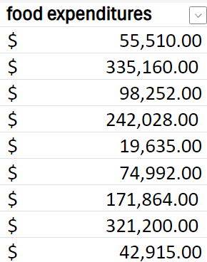
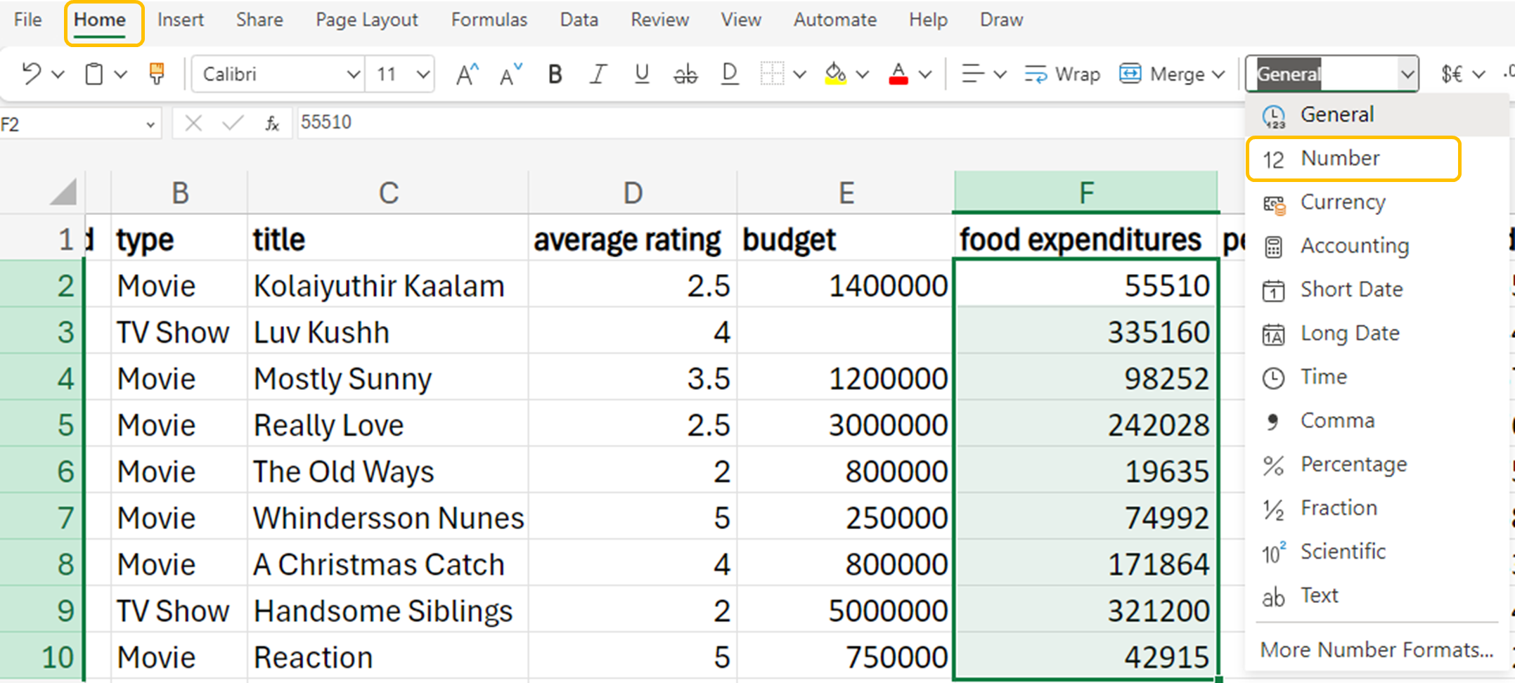
try it
Format the food expenditures column in accounting format by adding a dollar sign, two decimal places with the dollar sign, and decimal points in a column.

  1. Open netflix.xlsx.
  2. Select the food expenditures column.
  3. Select the drop-down arrow in the Number Format tool from the Home menu. Select Accounting.


    You should then see the food expenditures column update to the desired format.
  4. Check your work by comparing your formatted food expenditures column to the one in the example.

Number
Number formatting is used to display numbers with a specific amount of decimal places and without the thousands separators. For instance, formatting 1234.567 as a number with two decimal places would display it as 1234.57. Unlike Accounting though no dollar sign will be displayed.

EXAMPLE

In Excel, you can apply a number format. Number formatting applies two decimal places to the food expenditures column.
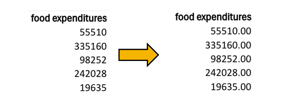
try it
Format the food expenditures column as a number with two decimal places.

  1. Open netflix.xlsx.
  2. Select the food expenditures column.
  3. Select the drop-down arrow in the Number Format tool from the Home menu. Select Number.


    You should then see the food expenditures column update to the desired format.
  4. Check your work by comparing your formatted food expenditures column to the one in the example.

did you know
You may have read the Comma and Number formatting definition and wondered if they are the same. The Comma format is a subset of the Number format with a predefined style that includes thousands separators and two decimal places by default. Both formats enhance the readability of numerical data, but the Comma format is specifically designed for the quick application of a standardized numeric presentation.

Percentage
The percentage format multiplies the cell value by 100 and displays the result with a percentage symbol. For example, if you enter 0.1234 and format it as a percentage with two decimal places, it will appear as 12.34%.

EXAMPLE

In Excel, you can apply a percentage format. Percentage formatting multiplies the highlighted cells by 100 and displays the results with a percent symbol (%) and two decimal places.

try it
Format the percent spent on food column in percentage format by multiplying by 100, adding a percent sign and two decimal places to the column.

  1. Open netflix.xlsx.
  2. Select the percent spent on food column.
  3. Select the drop-down arrow in the Number Format tool from the Home menu. Select Percentage.


    You should then see the percent spent on food column updated to the desired format.
  4. Check your work by comparing your formatted percent spent on food column to the one in the example.

All of these formatting tools help make numbers more readable and interpretable, ensuring numerical information is presented in a clear and professional manner.

2b. Formatting Text

Formatting text in Excel is essential for creating clear and visually appealing spreadsheets. For data analysts, getting data types and formats correct is fundamental to their work. It ensures:

  • Reliability: Accurate and reliable analysis results.
  • Efficiency: Streamlined data processing and manipulation.
  • Clarity: Clear and understandable reports and visualizations.
  • Collaboration: Smooth collaboration with team members and stakeholders.
Correct data types and formats are the backbone of effective data analysis. They help maintain data integrity, ensure accurate calculations, and facilitate efficient data manipulation and visualization.

Auto Fit
If you want to adjust the cell size to fit the text in the column or row, Auto Fit can greatly enhance the readability of your spreadsheet. You can manually adjust the column width and row height by dragging the borders of the column or row headers. Alternatively, you can use the Auto Fit feature to automatically resize the columns or rows to fit the text.

EXAMPLE

In Excel, you can apply the auto fit function. The auto fit function adjusts the column size to fit the longest string of text or numbers.
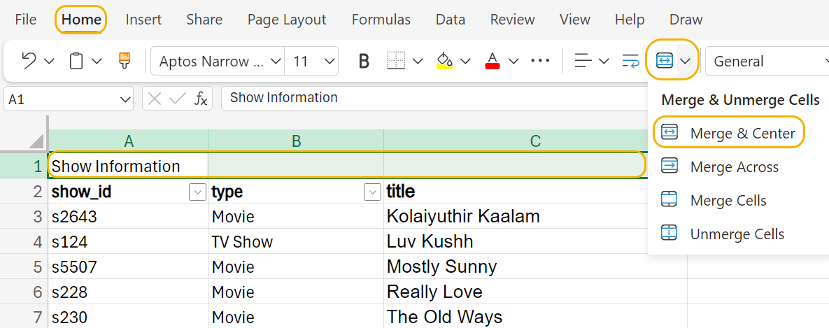
try it
Format the title column by adding two decimal places.

  1. Open netflix.xlsx.
  2. Select the title column.
  3. Go to the search window at the top of the Excel screen, type “Auto Fit Column Width,” then, choose “AutoFit Column Width.”


    You should then see the title column updated to the desired format.
  4. Check your work by comparing your formatted title column to the one in the example.

Merge and Center
Merge and center allow you to combine multiple cells into one larger cell and center the text within it. This is particularly handy for creating headers that span multiple columns.

EXAMPLE

Apply the merge and center function. The merge and center function allows you to center a title over multiple columns. Let’s create a heading that spans the first three columns of the data sheet, show_id, type and title. We can call this heading Show Information.

try it
Format the food expenditures column by adding two decimal places.

  1. Open netflix.xlsx.
  2. Select the first row of data and click the right mouse button.
  3. Choose “Insert Rows Above” to insert a row.


  4. Type “Show Information” in cell A1.


  5. Highlight cells, A1, B1, and C1, then choose (from the Home menu) the drop-down arrow to the right of Merge in the ribbon. Then, choose Merge & Center.


    You should then see the title column updated to the desired format.
  6. Check your work by comparing your formatted column to the one in the example.

2c. Formatting Dates

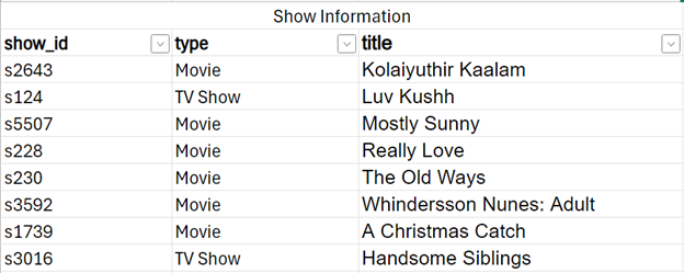
Data analysts need to work with consistent data. Consistency helps ensure data looks professional and can easily be sorted or filtered.

The Date format is used to display dates in various styles. Excel offers multiple date formats, such as MM/DD/YYYY, DD-MMM-YYYY, etc. For example, entering 07/13/2024 can be formatted to display as 13-Jul-2024.

EXAMPLE

In Excel, you can apply the date format to the date_added column to consistently format the date in MM/DD/YYYY format.

try it
Format the date_added column using date formatting.

  1. Open netflix.xlsx.
  2. Select the date_added column.
  3. Select the drop-down arrow to the right of the Number Format tool from the Home menu, then choose Short Date.


    You should then see the date_added column updated to the desired format.
  4. Check your work by comparing your formatted date_added column to the one in the example.

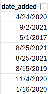
There are many different ways to format dates. By choosing the “Number Format” tool in the Home menu, scrolling to “More Number Formats...”, and then choosing the “Date” category, you can choose from many different date types from the window that appears on the right side of the screen.

In this window, one can find various other formatting options, or you can create your own by using the “Custom” feature.


3. Conditional Formatting

Conditional formatting in Excel is a powerful tool that allows you to automatically apply formatting to cells based on the values they contain. This feature is particularly useful for highlighting important data, identifying trends, and making your spreadsheet more visually appealing. With conditional formatting, you can set rules that change the appearance of cells, such as their background color, font color, or border, depending on the criteria you specify.

Another common use of conditional formatting is to create data bars, which visually represent the magnitude of values within a range. This can be particularly helpful for comparing numbers at a glance.

You can also use conditional formatting to create color scales, which apply a gradient of colors to a range of cells based on their values. For instance, you might use a color scale to highlight temperature data, with lower temperatures in blue and higher temperatures in red.

term to know
Conditional Formatting
An Excel tool that allows you to automatically apply formatting to cells based on the values they contain.

3a. Conditional Formatting with Numbers

A data analyst might use conditional formatting on numbers to quickly identify trends, outliers, and patterns within a dataset. By applying different colors, icons, or data bars to cells based on their values, conditional formatting helps to visually highlight important information, making it easier to spot anomalies or significant data points at a glance. This can be particularly useful when dealing with large datasets, as it allows the analyst to focus on key areas that require further investigation or action. Additionally, conditional formatting can enhance the overall readability and presentation of the data, making it more accessible and understandable for stakeholders who may not be as familiar with the raw numbers.

Apply Color to Numbers
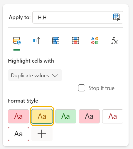
A data analyst might want to highlight all numbers above a certain threshold in yellow to quickly identify data.

EXAMPLE

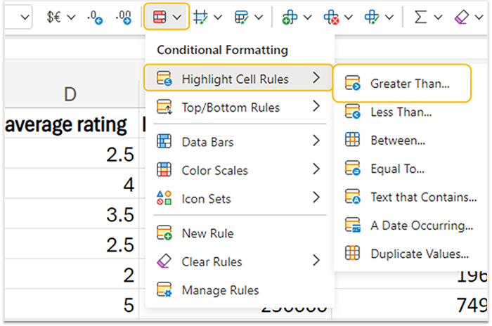
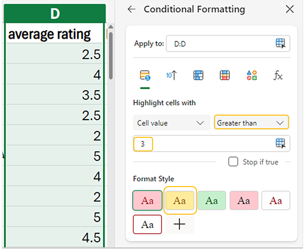
In Excel, you can apply conditional formatting to the average rating column to show which shows have an average rating of 3 or greater.

try it
Format the average rating column using conditional formatting to show which shows have an average rating of 3 or greater.

  1. Open netflix.xlsx.
  2. Select the average rating column.
  3. Select the drop-down arrow to the right of the Conditional Formatting tool from the Home menu. Hover over Highlight Cell Rules, and then choose Greater Than.


  4. In the Conditional Formatting window, on the right side of the document, choose the drop-down arrow next to Greater than. Then, choose Greater than or equals to. Type in the number 3 in the text window, and also choose the Yellow fill with dark yellow text tool under Format Style. Finally, click Done at the bottom of the window.


    You should then see the average rating column updated to the desired format.
  5. Check your work by comparing your formatted average rating column to the one in the example.

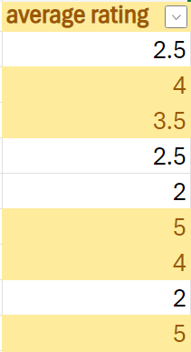
Highlight the Bottom 10%
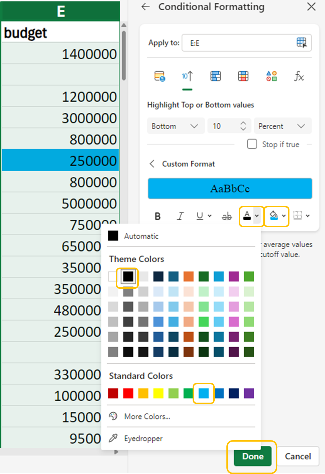
A data analyst might want to highlight all numbers below a certain threshold in light blue to pick out certain values quickly.

EXAMPLE

In Excel, you can apply conditional formatting to the budget column to see which shows have a budget in the bottom 10%.

try it
Format the budget column using conditional formatting to show which shows have a budget in the bottom 10%. Mark these in light blue font color.

  1. Open netflix.xlsx.
  2. Select the budget column.
  3. Select the drop-down arrow to the right of the Conditional Formatting tool from the Home menu. Hover over Top/Bottom Rules then choose Bottom 10%.


  4. In the Conditional Formatting window on the right side of the document, choose the drop-down arrow to the right of the Font Color tool and choose black. Then, select the drop-down arrow to the right of the Fill Color tool and choose light blue. Finally, click on Done.


    You should then see the budget column updated to the desired format. Items in light blue represent the bottom 10% of budget amounts.
  5. Check your work by comparing your formatted budget column to the one in the example.

3b. Conditional Formatting with Text

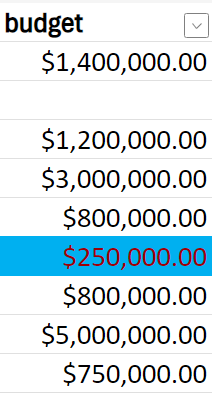
Much like using conditional formatting on numbers, you can use it on text to swiftly pinpoint and emphasize crucial information within a dataset. By setting up specific formatting rules, such as altering the font or background color based on certain conditions, analysts can detect patterns, anomalies, or significant categories. This visual distinction makes the data more comprehensible and accessible, facilitating quicker and more precise analysis. Moreover, conditional formatting can be employed to highlight errors or inconsistencies, ensuring the data’s quality and accuracy. In essence, it boosts the efficiency and effectiveness of data analysis by offering immediate visual indicators.

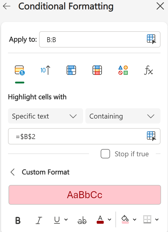
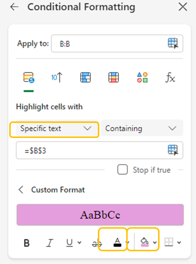
Highlight Movies and TV Shows in Different Colors
A data analyst might want to highlight all movies in blue and all TV shows in pink.

EXAMPLE

In Excel, you can apply conditional formatting to the type column so that all records that are movies are highlighted in light blue and all records that are listed as TV Show are highlighted in plum.
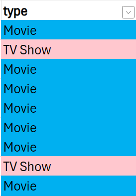
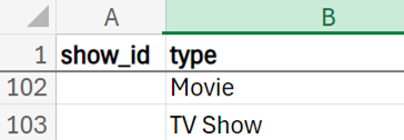
try it
Format the type column using conditional formatting to show records that are movies highlighted in light blue and all records that are listed as TV Shows are highlighted in plum, Accent 5, Lighter 60%.

  1. Open netflix.xlsx.
  2. Select the type column.
  3. Select the drop-down arrow to the right of the Conditional Formatting tool from the Home menu. Hover over Highlight Cell Rules then choose Text that Contains.


  4. In the Conditional Formatting window, on the right side of the document, click in the Input value or select a cell text box. Click in cell B2 or any cell that has the word “Movie” in it. Select the Custom Format (+) tool. This opens the Custom Format menu. Choose the drop-down arrow to the right of the Font Color tool and choose black. Then, select the drop-down arrow to the right of the Fill Color tool and choose light blue. Finally, click Done.


  5. In the Conditional Formatting window, on the right side of the document, select New Rule (+).


  6. Click on the drop-down arrow under Highlight cells with and select Specific Text. In the Input value or select a cell text box, click in cell B3 or any cell that has the words “TV Show” in it. Select the Custom Format (+) tool. This opens the Custom Format menu. Choose the drop-down arrow to the right of the Font Color tool and choose black. Then, select the drop-down arrow to the right of the Fill Color tool and choose plum. Finally, click Done.


    You should then see the type column updated to the desired format. Items in light blue represent Movies, and items in plum represent TV Shows.
  7. Check your work by comparing your formatted type column to the one in the example.

The UNIQUE Function
Suppose you want to highlight movies and TV shows differently using colors. You first need to examine the type column and determine what are the different categories of this categorical variable. You can use the UNIQUE() function in Excel.

When using the UNIQUE() function, there are some things to keep in mind. First is the syntax.

=UNIQUE(array, [by_col], [exactly_once]), where:

  • array is the range or array from which you want to extract unique values. This is the only required argument.
  • by_col is an optional argument. It is a logical value indicating how to compare values. By default, it compares by rows (FALSE). Set it to TRUE to compare by columns.
  • exactly_once is also an optional argument. It is a logical value that determines whether to return values that appear exactly once (TRUE) or all unique values (FALSE by default).
hint
For simple usages of the UNIQUE() function, meaning you only want to know how many unique identifiers are in a row or column, you would only need to choose the text you are interested in as the array (the first argument). The other arguments default to false.

EXAMPLE

You can apply the UNIQUE() function to the type column so you will know how many categories are in the data.

try it
Apply the UNIQUE() function to the type column to determine how many individual category types are listed in the data.

  1. Open netflix.xlsx.
  2. Navigate to the bottom of the type column and choose the cell below the last record. In this case, it is B102.
  3. In cell B102, type =UNIQUE(B2:B101). Alternately, you can also type in =UNIQUE(, then select the array you want, using the mouse. Do not forget to close the parentheses if you are using this method. Hit the Enter key.


    You should then see the list of unique values at the bottom of the type column. In this case, there are two unique types: Movie and TV Show.

3c. Conditional Formatting to Detect Duplicates

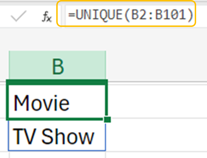
Conditional formatting in Excel provides a straightforward method to detect duplicates. The conditional formatting to detect duplicates does not alter the data, it just provides a visual cue for further action.

EXAMPLE

Identifying duplicate directors allows you to explore patterns. You might discover that some directors are prolific or that specific genres are associated with certain directors. Determining if there are any duplicate directors is the first step in this process.

You can use conditional formatting to detect that Garry Marshall is a director who appears twice in the Netflix data.

try it
Detect if the director column has any duplicate director names.

Open netflix.xlsx. Perform the following:

  1. Select the director column.
  2. Select the drop-down arrow to the right of the Conditional Formatting tool from the Home menu. Hover over Highlight Cell Rules then choose Duplicate Values.


  3. Select the Yellow fill with dark yellow text for the Format Style and click Done.


    You should see two highlighted rows (rows 56 and 84) that correspond to Garry Marshall.
  4. If you decided you wanted to remove the duplicate values from your data, under the Data Menu there is a Remove Duplicates option that removes the rows that contain the duplicated values.
  5. Check your work by verifying that you find two duplicated values of Garry Marshall in the director column.

summary
In this lesson, you learned how to format numbers, dates, and text in Excel to enhance data presentation and ensure consistency. Using a real-world dataset from Netflix, we explored various conditional formatting techniques. This included highlighting key information, such as differentiating TV shows from movies with distinct colors and identifying duplicates. Filtering will be further developed in the next lessons.

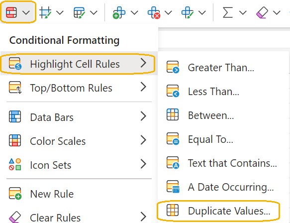
Source: THIS TUTORIAL WAS AUTHORED BY SOPHIA LEARNING. PLEASE SEE OUR TERMS OF USE.

Terms to Know
Conditional Formatting

An Excel tool that allows you to automatically apply formatting to cells based on the values they contain.