In this lesson, you will learn the fundamentals of exponential smoothing and how to apply the method for forecasting in Python. Specifically, this lesson will cover:
1. Introduction to Exponential Smoothing
Exponential smoothing is a technique used in business data analytics to forecast future data points by analyzing past data. Suppose you are a data analyst for a large retailer, and you want to predict next week's sales. You might look at the sales data from the past few weeks to make an educated guess. Exponential smoothing works in a similar way, but it gives more importance to recent sales data while still considering older data.
-
- Exponential Smoothing
- A forecasting technique that predicts future data points by giving more weight to recent data while still considering older data.
1a. Exponential Smoothing Calculation and Example
In exponential smoothing, each new forecast is made by combining the previous forecast and the most recent actual data point. The key idea is to apply a smoothing factor (usually a number between 0 and 1) that determines how much weight is given to the most recent data. A higher smoothing factor places greater importance on recent data, enabling the forecasts to adapt more swiftly to changing conditions in the data.
Simple exponential smoothing assigns more weight to recent data points through the smoothing factor (α). This weighting allows the forecast to adjust more quickly to changes in the data. When there is a sudden increase or decrease in the data, the exponential smoothing forecast will reflect this change more rapidly because it prioritizes the most recent data. This reduces the lag compared to moving averages, making exponential smoothing more responsive to new trends and shifts in the data.
To understand how exponential smoothing works, let's break down the calculation process step by step and illustrate it with a practical example.
To calculate an exponential smoothing forecast, follow these steps:
1. Identify the Time Period: Determine the time period for your data points, such as days, weeks, or months. This sets the context for your forecast.
2. Choose the Smoothing Factor: Decide on a smoothing factor (α), which is a number between 0 and 1. This factor determines how much weight is given to the most recent data point. A higher α gives more weight to recent data.
3. Calculate the Forecast: Use the formula:
-

where:
-
 forecast for the next period
- α = smoothing parameter
-
 actual value for the current period
-
 forecast value for the current period
4. Update and Repeat: After calculating the forecast for the next period, use it as the forecast for the current period in the next calculation.
Determining the optimal value of alpha (α) in exponential smoothing is always a challenge. Here are some common methods to find the best smoothing parameter.
-
Trial and Error: Start with a few different values of α (0.1, 0.3, 0.5, 0.7, 0.9) and compare the forecast accuracy measures (MSE, MAE, and MAPE) for each.
-
Domain Knowledge: Sometimes, understanding the nature of your data can help. If your data changes rapidly, a higher α (closer to 1) might be better. For more stable data, a lower α (closer to 0) might be more appropriate.
To grasp the idea of exponential smoothing, let’s walk through a simple example.
-
EXAMPLE
Suppose you have the following daily sales data for a week:
- Day 1: $100
- Day 2: $120
- Day 3: $130
- Day 4: $90
- Day 5: $150
- Day 6: $170
- Day 7: $160
Use a smoothing factor (α) of 0.4, since the last three days of sales are fairly stable (that is, not much variability).
Day 2 (


) Forecast: To initialize the calculations, set the forecasted value for time period 2 equal to the actual value of time period 1. So,

Day 3 (


) Forecast:

Day 4 (


) Forecast:

Day 5 (


) Forecast:

Day 6 (


) Forecast:

Day 7 (


) Forecast:

The table below shows the actual sales values and the forecasted values, based on exponential smoothing.
|
Day
|
Sales (Actual Data Values)
|
Exponential Smoothing Forecasts
|
|
Day 1
|
$100
|
|
|
Day 2
|
$120
|
$100 (initial forecast)
|
|
Day 3
|
$30
|
$108
|
|
Day 4
|
$90
|
$116.80
|
|
Day 5
|
$150
|
$106.08
|
|
Day 6
|
$170
|
$124.08
|
|
Day 7
|
$160
|
$142.45
|
Now, it is your turn to see if you can correctly apply the exponential smoothing technique to a small set of data.
-
Suppose you have the following weekly sales data for 5 weeks:
- Week 1: $500
- Week 2: $550
- Week 3: $600
- Week 4: $450
- Week 5: $700
Fill in the table below with the exponential smoothing forecasts for weeks 3-5.
Use a smoothing factor (α) of 0.80.
To initialize the calculations, set the forecasted value for week 2 equal to the actual value of week 1.
|
Week
|
Sales (Actual Data Values)
|
Exponential Smoothing Forecasts
|
|
Week 1
|
$500
|
|
|
Week 2
|
$550
|
$500 (initial forecast)
|
|
Week 3
|
$600
|
|
|
Week 4
|
$450
|
|
|
Week 5
|
$700
|
|
Solution:
|
Week
|
Sales (Actual Data Values)
|
Exponential Smoothing Forecasts
|
|
Week 1
|
$500
|
|
|
Week 2
|
$550
|
$500 (initial forecast)
|
|
Week 3
|
$600
|
$540
|
|
Week 4
|
$450
|
$588
|
|
Week 5
|
$700
|
$477.60
|
Week 3 (
) Forecast:

Week 4 (
) Forecast:

Week 5 (
) Forecast:

1b. Forecasting with Exponential Smoothing: Applications and Limitations
Exponential smoothing, similar to moving averages, are effective for short-term range forecasts, such as predicting the next time period. In a previous example, you calculated the exponential smoothing forecasts for sales data using the table below. The forecasted sales for Day 8 can be found by applying the exponential smoothing forecasting formula. A value of 0.40 was used for the smoothing parameter, α.
Day 7 (
 ) Forecast:

|
Day
|
Sales (Actual Data Values)
|
Exponential Smoothing Forecasts
|
|
Day 1
|
$100
|
|
|
Day 2
|
$120
|
$100 (initial forecast)
|
|
Day 3
|
$30
|
$108
|
|
Day 4
|
$90
|
$116.80
|
|
Day 5
|
$150
|
$106.08
|
|
Day 6
|
$170
|
$124.08
|
|
Day 7
|
$160
|
$142.45
|
|
Day 8
|
|
$149.47
|
Just like moving averages, exponential smoothing has limitations.
Below are some limitations of exponential smoothing to consider when deciding whether to use this method for forecasting:
-
Sensitivity to Smoothing Factor: The accuracy of the forecast heavily depends on the chosen smoothing factor (α). An inappropriate α can lead to inaccurate forecasts.
-
Best for Stable Data: Exponential smoothing works best with data that has a relatively stable mean and variance over time. This makes it suitable for stationary data where there are no significant trends or seasonal patterns.
Exponential smoothing is a powerful forecasting tool for relatively short-term forecasts for stationary data. However, its effectiveness diminishes when applied to data with significant trends or seasonal patterns. This is an important limitation to keep in mind when deciding whether to use this method for your forecasting needs. There are extensions of exponential smoothing that can address non-stationary data and data with seasonality, but they are beyond the scope of this tutorial.
2. Real-World Application of Exponential Smoothing in Python
In this section, you will explore how exponential smoothing can be applied in a real-world business scenario using Python.
2a. Forecasting with Exponential Smoothing
You are going to return to the same example you used in the previous tutorial to step into the shoes of a data analyst and use an exponential smoothing model to forecast monthly sales. Let’s begin!
-
EXAMPLE
Suppose you are a data analyst at TrendyBox, a subscription box service for trendy fashion accessories. Your task is to analyze the monthly sales data over the past two years (2023-2024) and forecast the sales for the next month (January 2025) using exponential smoothing in Python. Use an α value of 0.80. The data is here:
https://raw.githubusercontent.com/sophiaAcademics/BDA_Excel/main/StudentData/Tutorials/Unit5/5.2.4/trendybox_sales.xlsx
The code below imports pandas, imports an Excel file from a URL, and creates a pandas DataFrame named sales_es.
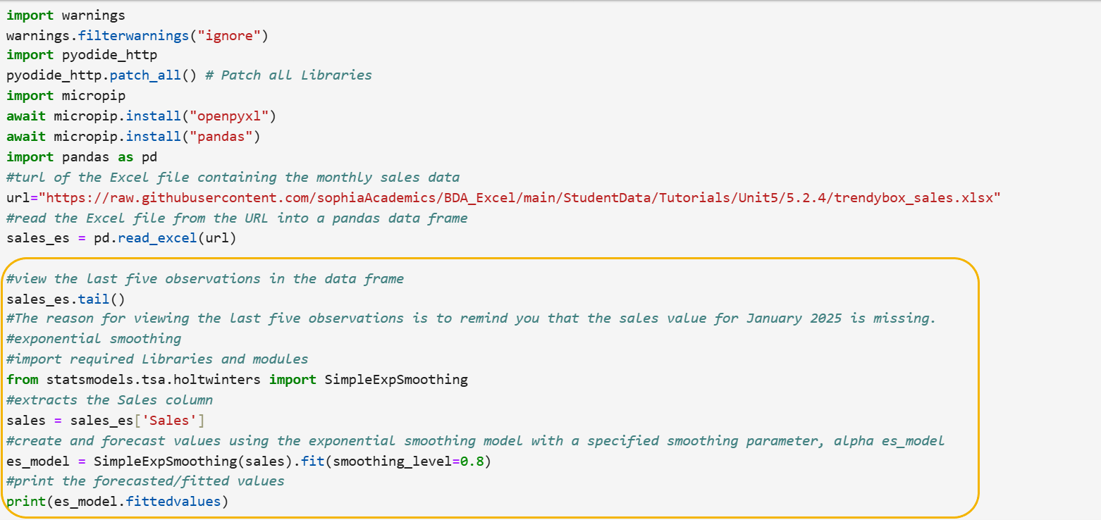
As shown, we now look at the tail() function, which shows us the last 5 rows of data.
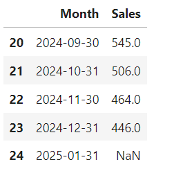
The reason for viewing the last five observations is to remind you that the sales value for January 2025 is missing. You will be forecasting this value using the exponential smoothing model.
In the statsmodels Python library, there is an exponential smoothing function that will perform exponential smoothing.
The code below imports the necessary Python library and modules, extracts the column in the DataFrame that contains the monthly sales data, creates an exponential smoothing model with a specified smoothing parameter of

and prints the forecasted values. Let’s look at the code line by line:
Step 1: Import the required Python libraries and modules.
from statsmodels.tsa.holtwinters import SimpleExpSmoothing
- This import statement allows you to use the SimpleExpSmoothing function in your code to create and forecast with an exponential smoothing model.
Step 2: Extract the column that contains the sales values.
sales = sales_es['Sales']
- This line extracts the Sales column from the sales_es DataFrame and assigns it to the variable sales.
Step 3: Apply the exponential smoothing model with a smoothing parameter of

es_model = SimpleExpSmoothing(sales).fit(smoothing_level=0.8)
- This line creates the forecasted values for sales using an exponential smoothing model with an α value of 0.80, meaning more importance will be given to the most recent monthly sales values.
The variable es_model holds the forecasted exponential smoothing values created using the SimpleExpSmoothing function and the sales data.
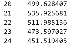
Step 4: Print the forecasted values.
print(es_model.fittedvalues)
- This line prints the exponential smoothing forecasts for each month.
The partial output below shows the last five values of the printed output. Notice that the 24th observation, which corresponds to January 2025, has a forecasted value of $451.52.
Now, it is your turn to practice forecasting with exponential smoothing in Python on your own!
-
You are going to return to the same scenario and data from the Try It exercise from the last tutorial.
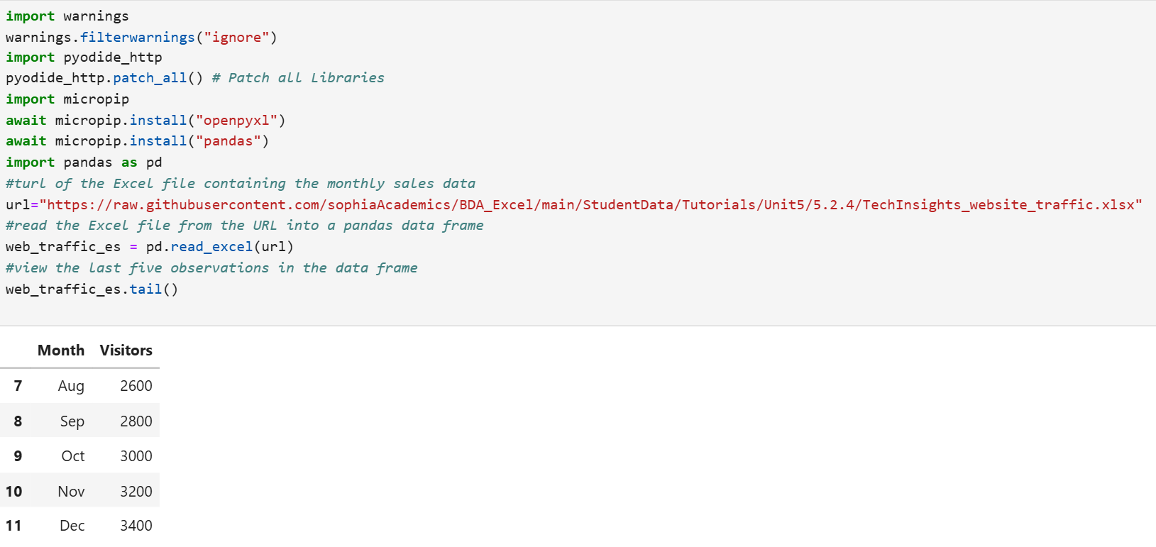
Suppose you are a data analyst at TechInsights, a tech blog that provides insights and updates on the latest technology trends. Your task is to analyze the monthly website traffic data (number of visitors to the website) over the past year (2024) and forecast the number of visitors for the next month (January 2025) using an exponential smoothing method in Python. Use an α value of 0.70.
The GitHub data is here:
https://raw.githubusercontent.com/sophiaAcademics/BDA_Excel/main/StudentData/Tutorials/Unit5/5.2.4/TechInsights_website_traffic.xlsx
Perform the following:
- Import the Excel file, create a pandas DataFrame named web_traffic_es, and view the last five rows of the DataFrame.
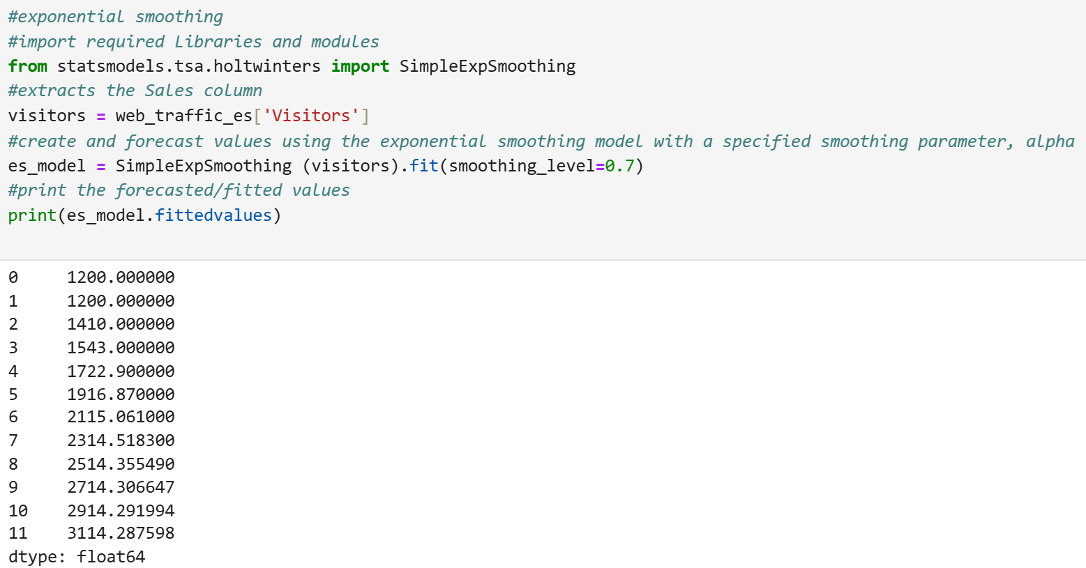
- Forecast the number of visitors for January 2025 using an exponential smoothing model with an α value of 0.70.
Solution:
1. The code below will create a pandas DataFrame named web_traffic_es and display the last five rows of the data.
2. The code below uses an exponential smoothing model with a smoothing parameter, α, of 0.70 to forecast the number of visitors that TechInsights can expect to visit their website in January 2025. The forecasted number of visitors in January 2025 is 3,114.
-
This video looks at forecasting the number of visitors using exponential smoothing.
2b. Exponential Smoothing Compared to Moving Averages
While both exponential smoothing and moving averages are used to smooth out fluctuations in data, they do so in different ways, and each has some similarities and some differences in their approach. The table below summarizes a comparison of key features of the two forecasting methods.
|
Feature
|
Moving Average
|
Exponential Smoothing
|
|
Weighting of Data
|
Equal weight to all data points in the window.
|
More weight to recent data points, due to α.
|
|
Adaptability
|
Slower to adapt to changes in the data.
|
Faster to adapt to changes in the data, due to α.
|
|
Complexity
|
Simple to calculate and understand.
|
Slightly more complex, due to α.
|
|
Best For
|
Short-term forecasts with stationary data.
|
Short-term forecasts with stationary data.
|
|
Initial Forecast
|
Not required.
|
Required so it can influence future forecasts.
|
|
Lag
|
Can lag behind actual data changes.
|
Less lag, due to α.
|
In this lesson, you learned how to calculate and apply exponential smoothing for forecasting. Exponential smoothing gives more weight to recent data while still considering older data, making it more responsive to changes in the data. You explored the step-by-step process of calculating exponential smoothing forecasts, including choosing the smoothing factor and updating forecasts, and practiced with a simple example of daily sales. The lesson also covered the applications and limitations of exponential smoothing, highlighting its effectiveness for short-term forecasts and its challenges with non-stationary data. You gained hands-on experience by implementing exponential smoothing techniques in Python using sales and website visitor data. A comparison of exponential smoothing and moving averages was provided to assist you in understanding the strengths and weaknesses of each method, helping you choose the most appropriate technique for your forecasting needs.