In this lesson, you will learn how to compute and evaluate the expected value and variance of a discrete random variable. Specifically, this lesson will cover:
1. Introduction to Expected Value and Variance
Expected value is essentially the average outcome you would expect from a set of probabilities. Imagine you have some dice, and you want to know the average number you would roll over many trials. The expected value helps you calculate this average.
In a business context, expected value can help you make informed decisions. For example, if you’re evaluating different investment opportunities, you can use the expected value to estimate the potential returns of each option. This way, you can choose the investment with the highest expected return. Imagine you are running an email marketing campaign and want to determine the expected revenue from this campaign. Expected value assists you in determining potential earnings from different marketing strategies.
Variance measures how much the outcomes of a discrete random variable differ from the expected value (the mean). In simpler terms, it tells you how spread out the numbers are. If the variance is high, the numbers are more spread out; if it's low, they are closer to the expected value. For example, you have collected data from several past email marketing campaigns and want to understand the variability in the revenue generated. A high variance would indicate that the revenue from the various email campaigns varies significantly from the mean. This suggests the outcomes are quite spread out, meaning the campaign performance is inconsistent. High variance in revenue might prompt you to investigate further. Are there specific factors causing some campaigns to perform much better or worse than others? Understanding these factors can help you reduce variability and achieve more consistent revenue generation from the email marketing campaigns.
-
- Expected Value
- Represents the average outcome of a discrete random variable if the process of generating the random variable was repeated many times.
1a. Discrete Probability Distributions
The foundation of expected value and variance is based on a discrete probability distribution. A discrete probability distribution lists all the possible values of a discrete random variable and its associated probabilities. Suppose you are analyzing the number of units sold per day for a new product. Based on historical data, you construct the following discrete probability distribution.
|
Units Sold (x )
|
Probability (P(x ))
|
|
0
|
0.10
|
|
1
|
0.20
|
|
2
|
0.30
|
|
3
|
0.25
|
|
4
|
0.15
|
In this scenario, the discrete random variable is the number of units sold. The Units Sold (x) column lists the possible outcomes for the discrete random variable. The Probability (P(x)) column shows the probability of each outcome occurring. For example, there is a 10% chance of selling 0 units, a 20% chance of selling 1 unit, and so on.
-
The lowercase
x value in a discrete probability distribution denotes the specific outcomes or values the discrete random variable can take on.
Notice that the sum of probabilities in the P(x) column sums to 1.0.

This ensures that one of these outcomes will occur, covering all possible scenarios for the number of units sold. In order for the probability distribution to be valid, the sum of the probabilities of a discrete probability distribution should always sum to 1.0.
Now, in a real-world business analytics scenario, you must use historical data to find and develop the discrete probability distribution. Let’s look at an example of how you would use Excel to develop a discrete probability distribution from historical data.
-
EXAMPLE
Suppose you have the number of complaints received each day from a company that services student loans.
The discrete probability distribution computed in Excel is provided below.
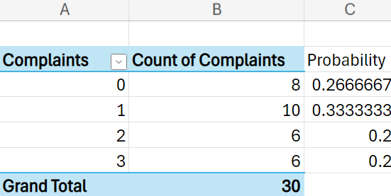
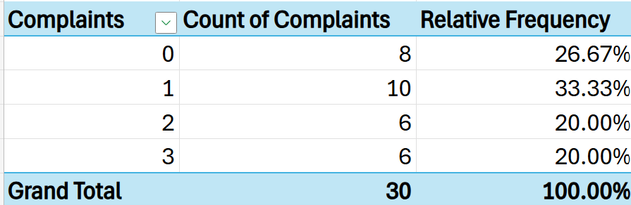
The student loan servicing company can use the discrete probability distribution to observe that the most likely number of complaints is 1 with a probability of 33.3%. The least likely number of complaints is 2 or 3 with a probability of 20% each.
-
Using the student loan servicing complaint data, construct the discrete probability distribution in Excel. The name of the Excel file is
student_loan_servicer_complaints.xlsx.
Using the student_loan_servicer_complaints.xlsx file, perform the following.
1. Select the entire range of your data (cells A1 to B31). On the
Insert menu, select
Pivot Table -->
From Table/Range and select +
New Worksheet. Place
Complaints in both the
Rows and Σ
Values box.
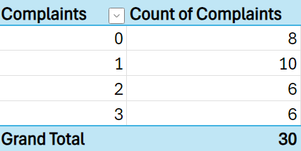
2. You need the values in the cells of the contingency table to represent the counts of each distinct number of complaints in the data (0, 1, 2, and 3). In the drop-down arrow for the Σ
Values box, select
Value Field Settings, select
Count, and
OK.
The PivotTable should update with the counts.
3. Add a new column to the PivotTable by entering the word
Probability in cell C2.
4. In cell C3, enter the formula:
=B3/$B$7
5. Once you have the formula entered in cell C3, hover over the small black plus sign (Auto-Fill Handle) at the bottom-right corner of the cell. Click and hold the left mouse button, then drag the handle down to cell C6.
6. The PivotTable should update to look like the one displayed in the previous example.

7. An alternate way to obtain the
Probability column is to create the
Relative Frequency column using the PivotTable functionality. Delete the
Probability column and put your cursor in the body of the PivotTable so you will have the
PivotTable Field options appear on the right-hand side of Excel. Drag
Complaints to the
Σ Values box. There will now be two instances of
Complaints in the
Σ Values box.
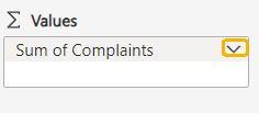
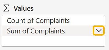
8. Using the drop-down arrow for the
Sum of Complaints in the
Σ Values box, select
Value Field Settings.
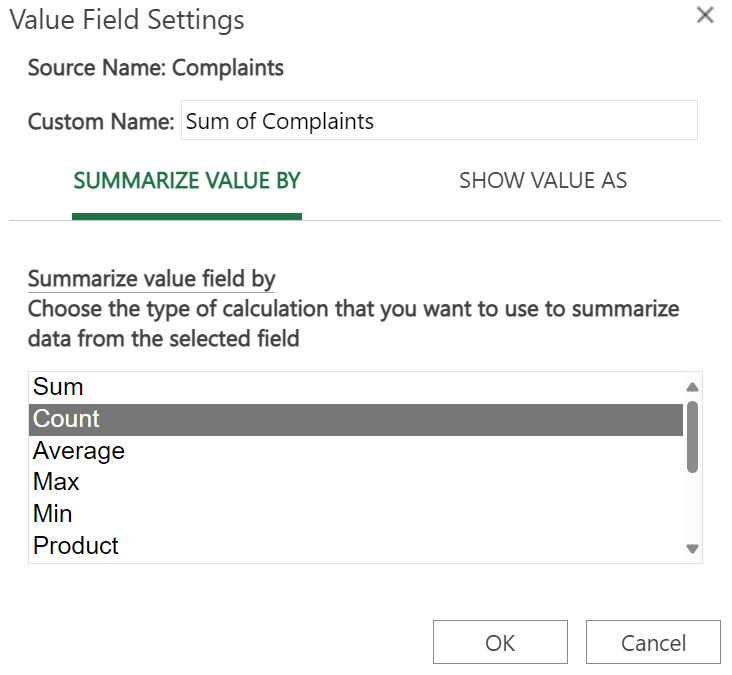
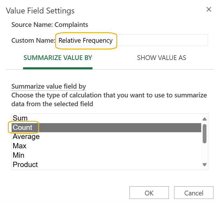
9. In the
Value Field Settings dialog box, name the new column
Relative Frequency and select
Count as the
SUMMARIZE VALUE BY.
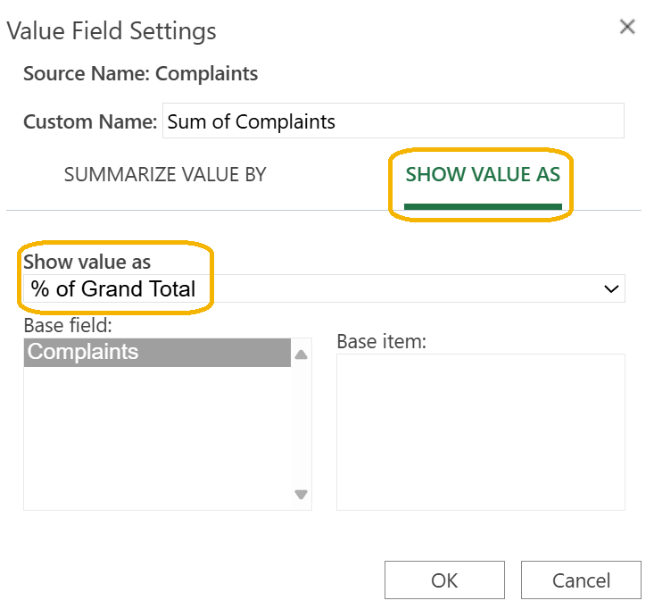
10. Select
SHOW VALUE AS, select
% of Grand Total, and select
OK.
You should now obtain a
Relative Frequency column in the PivotTable, which is the same as the
Probability column created previously.
11. Check your work by creating the discrete probability distribution in Excel.
-
Check out this video about constructing the discrete probability distribution.
-
- Discrete Probability Distribution
- Displays the probability of occurrence of each possible outcome of a discrete random variable.
1b. Expected Value
The expected value, denoted by  , of a discrete random variable is a measure of the central tendency, representing the average outcome if the business process or phenomenon were repeated many times. You calculate the expected value using:

where
x is the possible outcomes (numerical values) of the discrete random variable and

is the probability of observing a specific value of the discrete random variable.
Let’s take a look at an example calculation of expected value before you apply the concept to a real-world scenario.
-
EXAMPLE
Suppose you have the following probability discrete distribution.
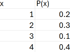
To find the expected value, use the formula:

This means that if the business process that generated the values of the discrete random variables and their associated probabilities were repeated many times, the average outcome would be 2.7.
Now, let’s apply the expected value to a real-world scenario.
-
EXAMPLE
You are assisting the director of marketing at UrbanHive, a company specializing in selling natural honey in urban areas. The director is keen to understand the effectiveness of their email marketing campaigns to optimize future strategies. Based on historical data, you have developed a discrete probability distribution that shows the revenue generated from the last five email marketing campaigns along with their associated probabilities.
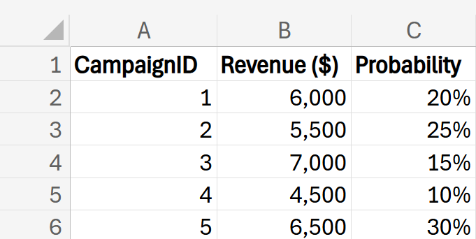
To provide insights to the director, you calculate the expected value as follows:

The expected revenue from the email marketing campaign is $6,025.
By calculating the expected value, you provide the director with a clear understanding of the average revenue that can be anticipated from future email marketing campaigns.
The director of marketing at UrbanHive can use the expected value of $6,025 in several ways to enhance decision-making:
-
Budgeting and Forecasting: The expected value provides a benchmark for future revenue from email marketing campaigns. This helps in setting realistic budgets and financial forecasts.
-
Performance Evaluation: The expected value serves as a performance metric. The director can compare actual campaign results against this benchmark to evaluate the effectiveness of different strategies and identify areas for improvement.
-
Communication with Management: The expected value provides a concrete figure that can be communicated to stakeholders, such as senior management or investors, to justify marketing expenditures and demonstrate potential returns.
-
Use Excel to compute the expected value of the revenue for the email marketing campaign for UrbanHive in the previous example.
Using the data in the
email_marketing_campaign.xlsx file, perform the following:
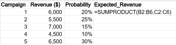
1. Create a new column by entering
Expected_Revenue in cell D1.
2. Enter the following formula in cell D2:
=SUMPRODUCT(B2:B6,C2:C6)
You should see the value 6025 populate cell D2.
The SUMPRODUCT() function in Excel simplifies the process of computing expected value by combining the multiplication and summation steps into a single function, making it both efficient and easy to use.
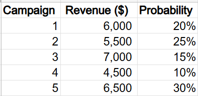
The function takes two arrays (ranges of cells) as inputs: B2:B6 (the values of the random variable,
x) and C2:C6 (the corresponding probabilities
). It multiplies each element in the first array by the corresponding element in the second array. After multiplying the corresponding elements, the function sums the products together. So, it is performing the expected value calculation.
The screenshot below shows the Excel formula.
1c. Variance
The variance of a discrete random variable, denoted as Var(x), is a measure of how much the values of the random variable deviate from the expected value (mean). It indicates the spread or dispersion of the values. You calculate the variance using:

where
x is the numerical outcome of the discrete random variable,

is the expected value (mean) of the discrete random variable, and
is the probability of observing a specific value of the discrete random variable.
The squared difference between each value of the discrete random variable and its mean is multiplied by each corresponding probability.
The relationship between variance and standard deviation also applies to discrete random variables. To find the standard deviation of a discrete random variable (X), you simply take the square root of its variance, 
Let’s look at an example calculation of expected value before you apply the concept to a real-world scenario.
-
EXAMPLE
Suppose you have the following probability discrete distribution from the previous section. Remember that the expected value was 2.7.

To find the variance, use the formula:

Let’s return to assisting the director of marketing and provide some insight into the email marketing campaign by applying variance.
-
EXAMPLE
Let's return to the scenario where you are assisting the director of marketing at UrbanHive, a company specializing in selling natural honey in urban areas. You have learned that variance is another measure that can be computed from a discrete probability distribution. You decide to compute the variance for the last five email marketing campaigns and provide the director with some insights using variance.
Recall the expected value of the revenue was $6,025 from the previous example.
To calculate variance, perform the following:

The variance of $511,875 indicates the degree to which the revenues from the email marketing campaigns deviate from the mean revenue of $6,025. This information can help the director of marketing use the variance information in several strategic ways to make informed decisions, such as:
-
Assessing Risk and Stability:
-
High Variance: High variance indicates that the revenues from the campaigns are widely spread out from the mean. This means there is a significant difference between the best and worst-performing campaigns.
High variance indicates that the revenues from the campaigns are highly variable. This suggests that some campaigns perform very well while others do not, which could be risky. The director might want to investigate the factors contributing to this variability and work on strategies to stabilize the performance.
-
Low Variance: Low variance indicates that the revenues from the campaigns are closely clustered around the mean. This suggests that the revenues are more consistent across campaigns. This stability can be reassuring and might indicate that the marketing strategies are generally effective.
In the context of evaluating the performance of marketing campaigns, what is considered “high” or “low” variance can depend on several factors, including industry standards, company goals, and historical performance data.
-
Understanding Customer Preferences: High variance might indicate that different campaigns resonate differently with various customer segments. Analyzing these differences can provide insights into customer preferences and help tailor future campaigns more effectively.
-
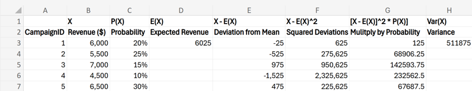
Use Excel to compute the variance of the revenue for UrbanHive's email marketing campaign.
Using the data in the
email_marketing_campaign.xlsx file, perform the following.
1. Create a new column by entering
Deviation from Mean in cell E2.
2. Enter the following formula in cell E3:
=B3-$D$3
Drag this formula down to cell E7.
3. Create a new column named
Squared Deviations in cell F2.
4. Enter the following formula in cell F3:
=E3^2
Drag this formula down to cell F7.
The symbol ^, pronounced "caret," is the exponent symbol in Excel.
5. Create a new column named
Multiply by Probability in cell G2.
6. Enter the following formula in cell G3:
=F3*C3
Drag this formula down to cell G7.
7. Sum up all the values in column G to calculate the variance. In cell H2, create a new column named
Variance and enter the following formula in cell H3:
=SUM(G2:G6)
8. You should see the value 511875 populate cell H3.
The formulas used in Excel are shown below, along with the actual values that the formulas produced.
-
Follow along with this video to compute the variance for the revenue for the email marketing campaign.
In this lesson, you focused on the ideas of expected value and variance for a discrete random variable. The expected value (or mean) of a discrete random variable is a measure of the central tendency of a discrete probability distribution. In a business data analytics context, expected value helps in predicting the average outcome of a random event based on historical data. For example, the expected value calculation of several past marketing campaigns for UrbanHive assisted the director of marketing in understanding the average revenue that can be anticipated from future email marketing campaigns. The revenue stability of the email marketing campaigns was assessed through variance. The variance calculation for the email marketing campaigns provides the director of marketing with insights into the consistency and risk associated with the revenue generated from these campaigns.