Table of Contents |
As consumers, we are always searching for what we want at a price we are willing to pay, which is the essence of demand.
At the same time, producers want to provide us with goods at prices we will pay, because that is the only way that they will make money. Therefore, producers focus on supply.
Let’s briefly review the laws of supply and demand.
The law of demand is the inverse correlation between price and quantity, with all other variables being fixed.
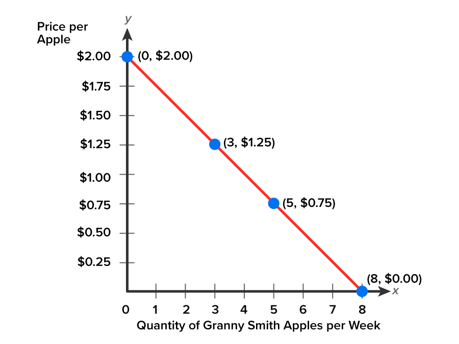
Here is a demand schedule for Granny Smith apples outlining how many apples a consumer would purchase at different prices.
| Price of Granny Smith Apples | Quantity of Granny Smith Apples Each Week |
|---|---|
| $2.00 | 0 |
| $1.75 | 1 |
| $1.50 | 2 |
| $1.25 | 3 |
| $1.00 | 4 |
| $0.75 | 5 |
| $0.50 | 6 |
| $0.25 | 7 |
| $0.00 | 8 |
When we plot the points, we can see the inverse relationship between price and quantity. As the price of apples goes down, we buy more. As the price of apples goes up, we move along the curve to buy fewer apples.
Therefore, there is a negative relationship between price and quantity with demand.
Now, the law of supply states that if the price of a good decreases, the quantity supplied decreases. The opposite would also be the case, meaning that as prices go up, the quantity supplied would also increase.
Again, using the same prices for apples, now you can see a different relationship between price and quantity.
| Price of Granny Smith Apples | Quantity of Granny Smith Apples Each Week |
|---|---|
| $2.00 | 7 |
| $1.75 | 6 |
| $1.50 | 5 |
| $1.25 | 4 |
| $1.00 | 3 |
| $0.75 | 2 |
| $0.50 | 1 |
| $0.25 | 0 |
As the price goes down, the quantity these farmers are willing to produce falls. As the price goes up, the quantity that they are willing and able to produce rises. This represents a positive relationship between price and quantity for supply.

Now, equilibrium involves putting supply and demand together, looking at how buyers (demand) and sellers (supply) come together in the market.
We know that consumers want low prices. We also know that producers would love to sell at high prices. So, how do they agree on a price?
Let’s look at both the schedule of supply and demand and the corresponding graph. Notice that demand is shown in green, while supply is indicated in red.
| Price of Apple | Quantity of Apples Supplied | Quantity of Apples Demanded |
|---|---|---|
| $2.00 | 7,000 | 0 |
| $1.75 | 6,000 | 1,000 |
| $1.50 | 5,000 | 1,500 |
| $1.25 | 4,000 | 2,000 |
| $1.00 | 3,000 | 3,000 |
| $0.75 | 2,000 | 4,000 |
| $0.50 | 1,000 | 5,000 |
| $0.25 | 0 | 6,000 |

At prices at $1.00: Qs = Qd
At prices below $1.00: Qd > Qs
As you likely determined, the point at which these two graphs meet is, in fact, equilibrium. However, let’s examine how we get to this point.
Notice that at any price above $1, the quantity supplied exceeds the quantity demanded.
| Price of Apple | Quantity of Apples Supplied | Quantity of Apples Demanded |
|---|---|---|
| $2.00 | 7,000 | 0 |
| $1.75 | 6,000 | 1,000 |
| $1.50 | 5,000 | 1,500 |
| $1.25 | 4,000 | 2,000 |
| $1.00 | 3,000 | 3,000 |
| $0.75 | 2,000 | 4,000 |
| $0.50 | 1,000 | 5,000 |
| $0.25 | 0 | 6,000 |
This means that at prices above $1, many farmers want to grow apples. However, people do not want to buy these many apples at those prices. Therefore, there are many more apples available for sale in grocery stores than people willing to purchase them. At those higher prices, then, the quantity supplied exceeds the quantity demanded.
As the price falls, we are getting closer to the point of equilibrium, but we can still see that the quantity supplied is greater than the quantity demanded.
The grocers will respond by lowering the price to entice consumers to buy—otherwise, the apples will spoil. Now that the apples are being sold at a lower price, the farmers will also need to react. Perhaps next month, some of the farmers will decide to produce something else, because they do not want to produce something that is lowering in price. Effectively, their incentive has been taken away.
As the law of supply dictates, farmers have an incentive to produce more as the price goes up and less as the price goes down. Therefore, as the price falls, we know that the quantity demanded rises, while the quantity supplied falls. As the price comes down, these two will converge until equilibrium is reached.
Now, let’s look at the opposite situation—prices below $1. In this case, if the price fell too much or the price started too low, the quantity demanded would now exceed the quantity supplied.
| Price of Apple | Quantity of Apples Supplied | Quantity of Apples Demanded |
|---|---|---|
| $2.00 | 7,000 | 0 |
| $1.75 | 6,000 | 1,000 |
| $1.50 | 5,000 | 1,500 |
| $1.25 | 4,000 | 2,000 |
| $1.00 | 3,000 | 3,000 |
| $0.75 | 2,000 | 4,000 |
| $0.50 | 1,000 | 5,000 |
| $0.25 | 0 | 6,000 |
Now that apples are so cheap, more consumers want to purchase them. However, because of the low price, there are not as many available for sale, because farmers have not produced them at those low prices. Therefore, grocers are selling out.
Now, because they are selling out, grocers have the incentive to raise prices. They see that people are demanding the apples, yet the grocers do not have enough to meet the current supply.
At the higher price, some farmers now have the incentive to get back into the market, or more people will enter the market and the quantity supplied will rise. At the same time, as prices are on the rise, we know that the quantity demanded will fall.
Once again, the two will converge until we meet at equilibrium or the prevailing price.
Now, you can see here that the only price at which the quantity supplied and the quantity demanded are equal is $1. The price of $1 clears the market, which means that every buyer has a seller, and every seller has a buyer.
| Price of Apple | Quantity of Apples Supplied | Quantity of Apples Demanded |
|---|---|---|
| $2.00 | 7,000 | 0 |
| $1.75 | 6,000 | 1,000 |
| $1.50 | 5,000 | 1,500 |
| $1.25 | 4,000 | 2,000 |
| $1.00 | 3,000 | 3,000 |
| $0.75 | 2,000 | 4,000 |
| $0.50 | 1,000 | 5,000 |
| $0.25 | 0 | 6,000 |
At this point of equilibrium, there is no tendency for change. There is no incentive to raise or lower the price.
Equilibrium, then, is defined as the price and quantity pair at which supply and demand intersect; in other words, it is the price and quantity at which the market clears.
Source: THIS TUTORIAL WAS AUTHORED BY KATE ESKRA FOR SOPHIA LEARNING. PLEASE SEE OUR TERMS OF USE.