Let's begin with a quick review of the laws of supply and demand:
In this tutorial, we will be discussing exactly how much more or less, and if it is the same for every good.
Elasticity is the measurement of the change in quantity demanded or supplied which indicates the sensitivity of one variable to characteristics of another variable or income.
In other words, how much do people respond--by buying or supplying more/less--when something else changes, like the price of the good itself, the price of a related good, or people's income?
The answer is that it really depends on the good or service:
Let's explore some examples to illustrate the different measurements of elasticity.
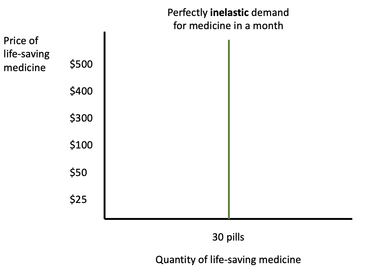
This reflects perfectly inelastic demand for a life-saving medicine. Notice that no matter what the price, this consumer is buying the exact same quantity--30 pills per month. Therefore, they are not responsive at all to a price change because a life-saving medicine is a necessity, and there are no substitutes.
This is not straight up and down, or completely vertical, because people do change their behavior somewhat as the price of gasoline goes up.
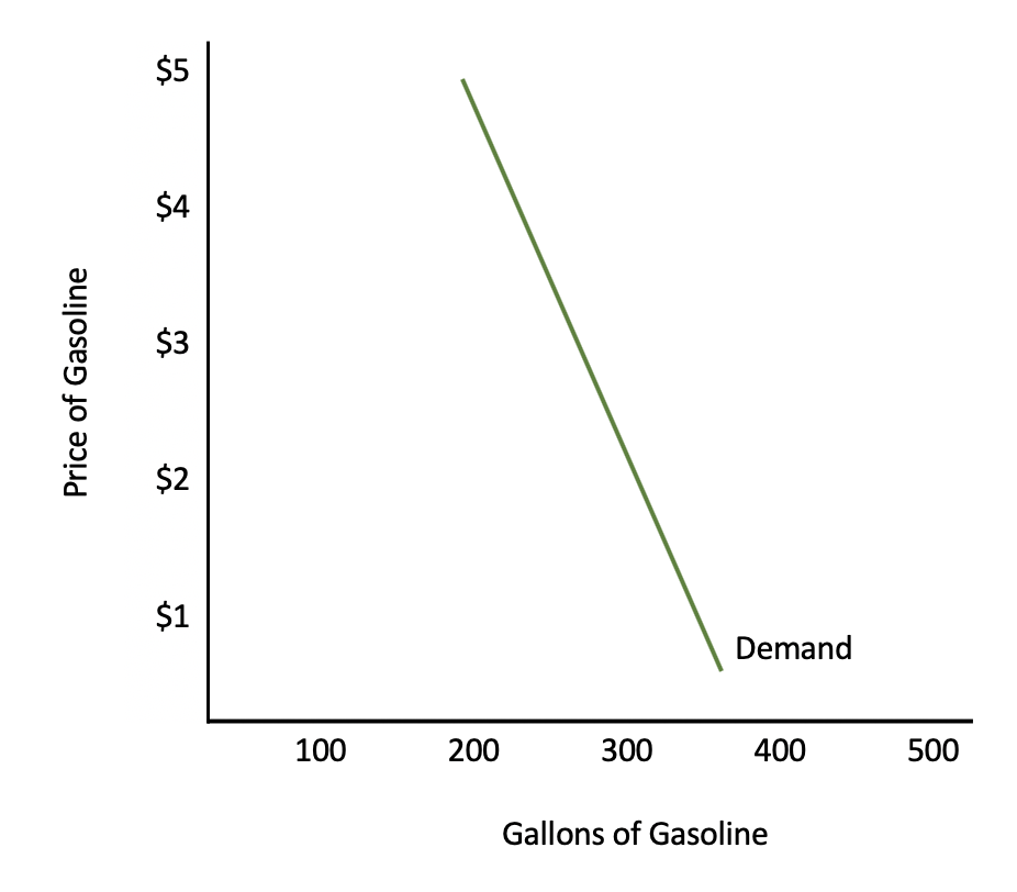
However, notice how the price can change significantly, yet consumers do not change their purchasing habits very much. This is because most people view gasoline--at least in the short term--as a necessity.
We will use the example of a hot dog stand that is one of 200 stands in a baseball stadium. They are all selling an identical product and are all charging $5 for that identical hot dog.
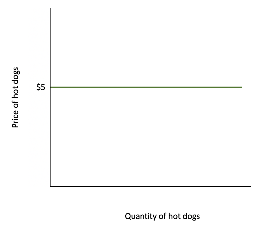
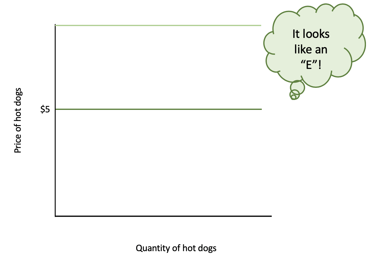
If one hot dog stand out of 200 decided to raise price up to $6, for instance, no one would purchase a hot dog there. The quantity demanded, in theory, according to this curve, would drop to zero, which is what a completely horizontal demand curve would imply--it is perfectly elastic.
Demand for a specific type of apples, like Gala apples, would be somewhat elastic.
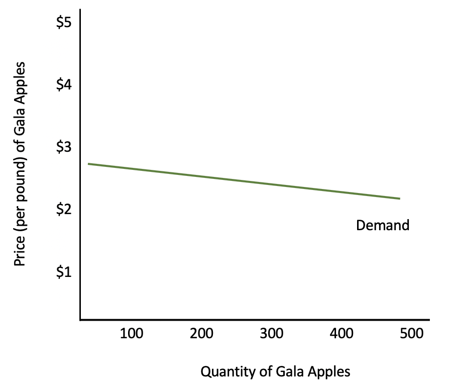
It is not completely horizontal, because prices could increase a bit and you would still see purchases of Gala apples by people who simply prefer them.
However, quite a few people would change their minds. Notice how quantity is changing significantly compared to price because there are so many substitutes for Gala apples.
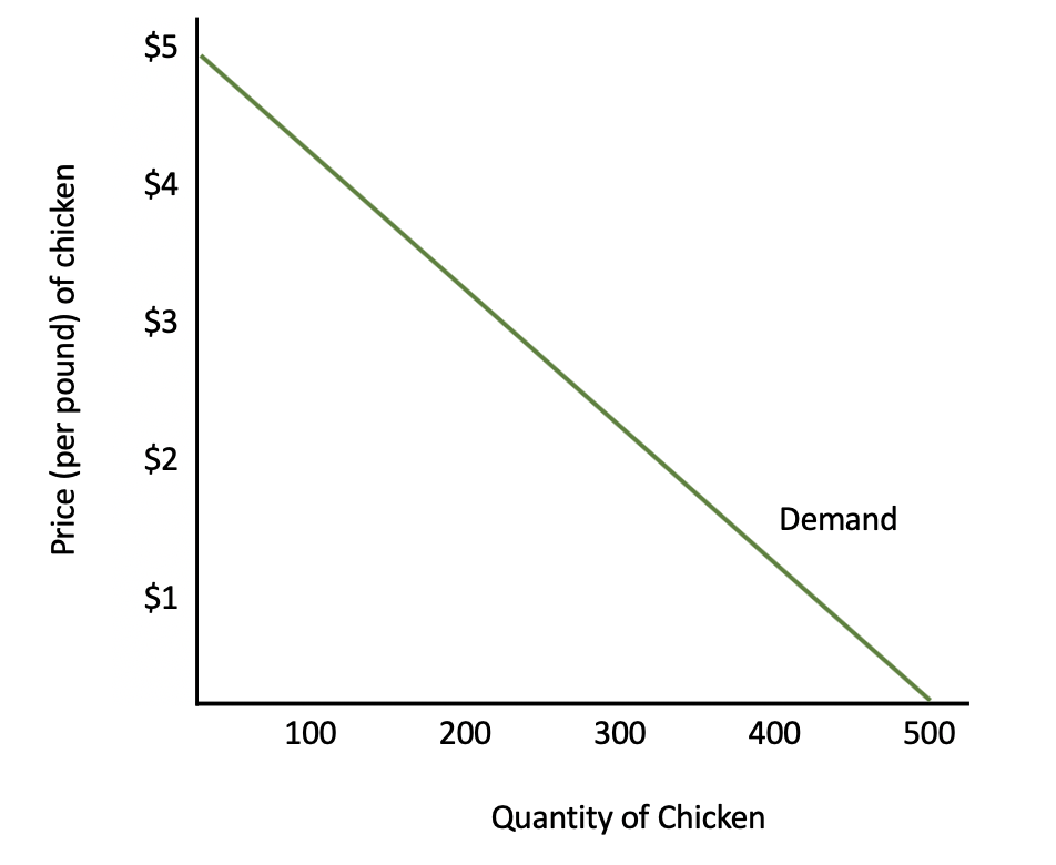
Along this curve, let's assume that the price of chicken rises by 10%, and as a result, consumers buy exactly 10% less chicken. This means that the proportion of how much people respond is identical to the percentage change in price. In other words, people's response is proportional to the percentage change in price.
All of these examples involve own-price elasticity, which is elasticity of either demand or supply when the price of a good changes, keeping all other variables and goods separate.
To fully understand the concept, let's walk through an example.
Is bottled water at the zoo elastic or inelastic in demand? Suppose the zoo was selling bottled water for $2, and they were selling 500 bottles of water a day.
The zoo decides to raise prices to $4 per bottle of water, and now they are selling 400 bottles of water a day.
The equation for elasticity is the percentage change in quantity-- how much people respond--divided by the percentage change in price.

| Elasticity Equation | |
|---|---|
| For Demand | For Supply |
| NEGATIVE, since Q & P move in opposite directions | POSITIVE, since Q & P move in the same direction |
For this example, we are only concerned about absolute value for own-price elasticity. We are simply looking at two points along the demand curve for water at the zoo to compare the change in quantity to the change in price (arc price elasticity).
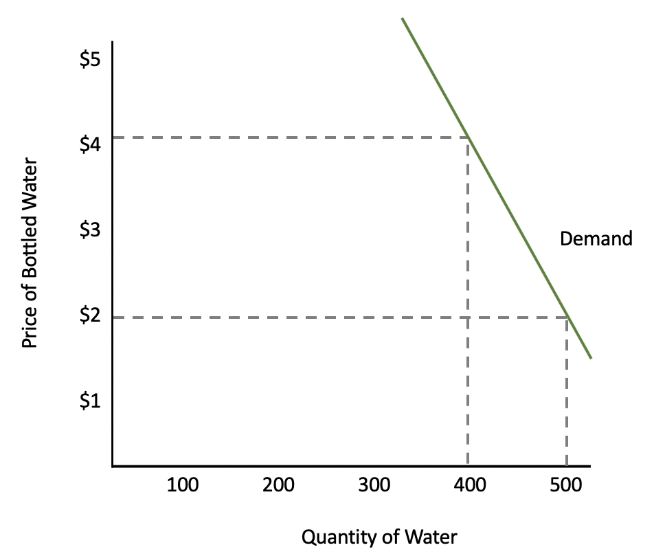
Let's plug our numbers into the elasticity equation. Note that the absolute change from 500 bottles to 400 bottles is 100 bottles and the absolute change from $2 to $4 is $2.

Our elasticity coefficient is 0.20, but what does this number mean?
Well, when we look at the elasticity coefficient for own-price elasticity, a coefficient greater than 1 indicates that demand would be elastic because that would suggest that the numerator responds more than the denominator. So, people change their buying habits by more than the percentage change in price.
Inelastic demand results in a coefficient less than 1 because people are not as responsive to the change in price.
Unit elastic is when the two change proportionately, with an elasticity coefficient equal to 1.
| Price Elasticity Coefficients | |
|---|---|
| E > 1 | Elastic Demand/Supply |
| E < 1 | Inelastic Demand/Supply |
| E = 1 | Unit Elastic Demand/Supply |
Now, cross-price elasticity is a change of demand or supply that occurs due to a change in the price of substitutes or complements.
To illustrate, let's look at an example using the brands Nike and Adidas. We are going to look at what will happen to the quantity of Nike, not when the price of Nike changes, but when the price of Adidas changes.
| Quantity of Nike Shoes | Price of Adidas Shoes |
|---|---|
| QA = 200 | PA = $110 |
| QB = 240 | PB = $130 |
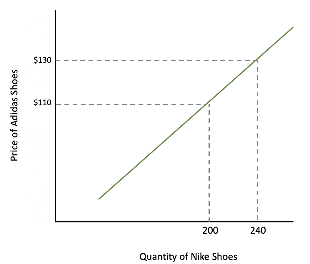
Let's plug our numbers into the elasticity equation.

If we perform the calculation, we get a cross-price elasticity of 1.1.
In this case, it does matter what direction price and quantity are moving. We are not just looking at the absolute value, because with cross-price elasticity:
In this case, with a positive 1.11 coefficient, Nike and Adidas must be substitutes. When Adidas raises prices, people will buy more of a substitute, like Nike.
| Cross-Price Elasticity Coefficients | |
|---|---|
| E < 0 | Complements |
| E > 0 | Substitutes |
Finally, let's discuss our last type of elasticity, income elasticity. Income elasticity is an economic measure of change in relation to income and demand for normal, inferior, and luxury goods.
Continuing with Nike as an example, if our incomes rise, will we buy more or less Nike apparel?
For example, Tom's income increases from $20,000 to $40,000. He used to buy two pairs of Nike running shoes a year, but now he can afford to buy three pairs.
| Quantity of Nike Shoes | Income |
|---|---|
| QA = 2 Pairs | IA = $20,000 |
| QB = 3 Pairs | IB = $40,000 |
Tom's demand curve is shown below. Notice, though, that instead of looking at what happens when the price changes, we are looking at what happens when someone's income changes.
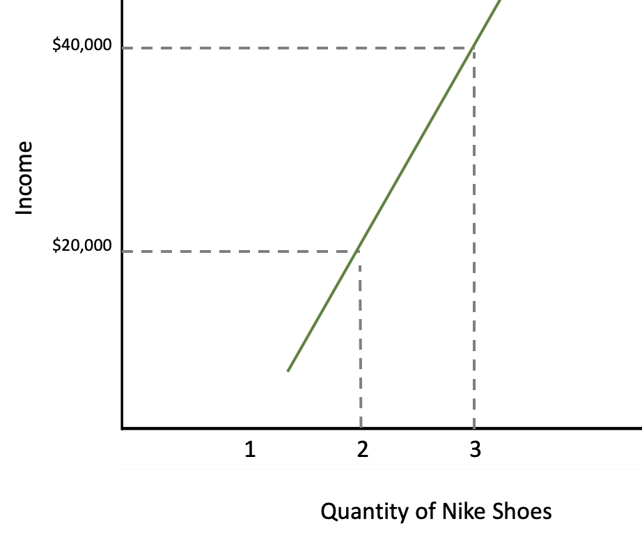
As you can see, there is a positive relationship between income and Nike shoes purchased.
Let's plug our numbers into the elasticity equation.

Performing the calculations, we see that we get an elasticity coefficient of a positive 0.50.
Again, the coefficient does matter in terms of the sign; it is not just absolute value. Therefore, that positive 0.50 tells us that the good is a normal good. If the coefficient were negative, the good would be an inferior good.
Vacations are another example of a normal good or something we buy more of as our income goes up. Notice how when your income is $40,000, you are able to go on one vacation, whereas when your income is $80,000, you might go on three vacations in a year.
| Quantity of Vacations | Income |
|---|---|
| QA = 1 | IA = $40,000 |
| QB = 3 | IB = $80,000 |
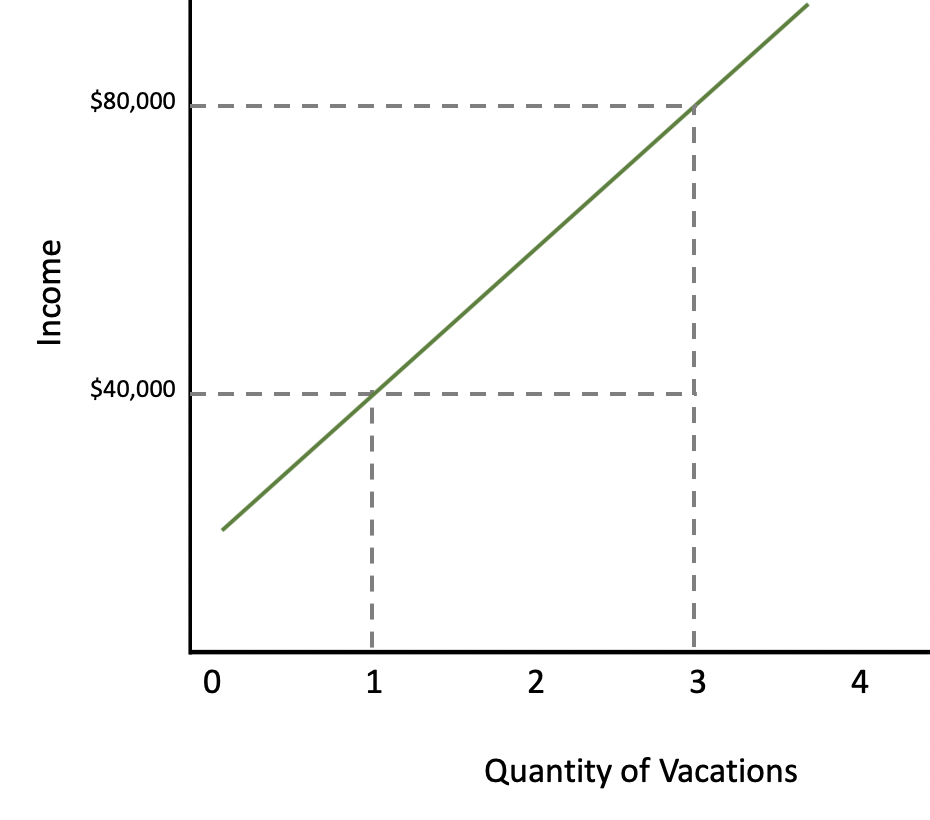
Let's plug our numbers into the elasticity equation.

The coefficient, if you plug the numbers in, would be a positive 2, which would indicate that vacations are a normal good.
A luxury good defined is a good that offers better quality and features which is consumed when income rises.
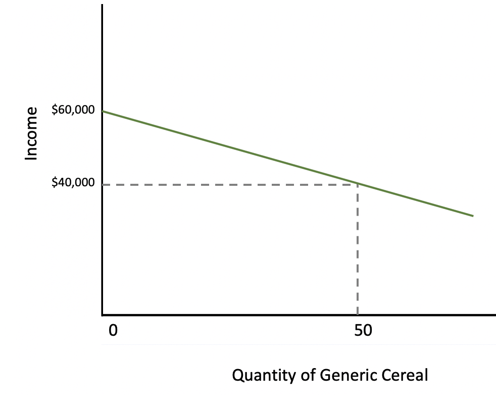
For the above example, let's plug our numbers into the elasticity equation.

The coefficient is negative, which indicates an inferior good, or one for which demand decreases as income increases.
| Income Elasticity Coefficients | |
|---|---|
| E < 0 | Inferior Good |
| E > 0 | Normal Good |
| E > 1 | Luxury Good |
Source: Adapted from Sophia instructor Kate Eskra.