Distributions for Quantitative Data

1. Distributions for Quantitative Data

Frequency distributions for quantitative variables can also be constructed, but the approach compared to categorical variables is different. The approaches are different because the measurement levels are different for each data type. For example, a categorical variable’s values are represented as distinct categories. Whereas, a quantitative variable’s values are represented as numeric values that can be continuous (can take on a value in an interval) or discrete.

To construct a frequency distribution for a quantitative variable, you create groups, also known as bins, that divide the data into a range of intervals. You then count how many observations fall within each bin. These bins allow you to see all the possible values of the quantitative variable. The tabular creation of the bins and the count of values that fall within each bin is how you construct a frequency distribution for a quantitative variable. These bins also serve as the foundation for constructing a histogram. A histogram allows you to visualize the distribution of the quantitative variable for both continuous and discrete measurement levels.

think about it

Why didn’t we need to create bins in the previous tutorial covering categorical variables?

Categorical variables have natural categories, so there is no need, nor is it possible, to create intervals for grouping those data, i.e. bins.

terms to know

Bins

Specific interval or range of values in which data is grouped.

Histogram

The visualization of a frequency distribution for a quantitative variable.

2. Frequency Distributions and Histograms to Detect Potential Outliers

The procedure for creating a distribution for a quantitative variable is to group the data into equally spaced intervals and then count how many observations fall within each bin. Before you begin, you must make some decisions, such as:

1. How many bins should we use?
2. How wide should our bins be?

For example, imagine you have a quantitative variable with very little variation in its values. If you use too many narrow bins, each bin captures only a small range of the data values. Even minor fluctuations within that range appear as significant peaks or valleys in the distribution. The histogram will be jagged when the frequency distribution is visualized because of these exaggerated fluctuations. Instead of a smooth curve representing the true distribution, you see a series of sharp spikes and dips. You might interpret these spikes as meaningful features of the data. When in fact, the spikes are just a function of the narrow bins that were created due to having too many bins.

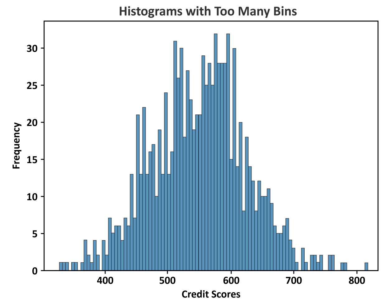
Another issue with too many bins is that some bins may have no observations, causing there to be gaps in the distribution, which provides no information. The figure below illustrates a histogram for an individual’s credit scores. A credit score is a discrete value that can range from 300 to 850. A higher credit score generally indicates better financial health and credit management. The histogram has too many bins. The excessive bins make it difficult to visually interpret the data. The histogram is cluttered and choppy so your ability to detect any patterns is hindered.

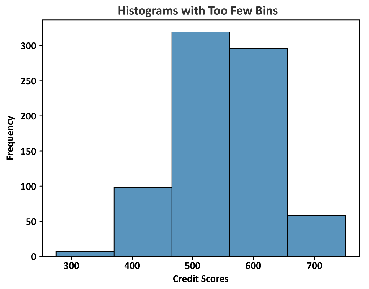
You can also run into issues if you select too few bins when constructing the frequency distribution. Too few bins can lead to oversimplification of the distribution. You may not pick up on certain nuances of the data or the general pattern of the distribution. The histogram created from the limited number of bins may mislead you by not accurately reflecting important fluctuations or variations in the data. The figure below illustrates the distribution of credit scores when the histogram has too few bins. Using this histogram, you might overlook specific score ranges that are critical for decision making. For example, identifying creditworthy applicants.

There are some rules of thumb that have been created for determining the number of bins for a frequency distribution for a quantitative variable and ultimately for the histogram.

The square root rule states that the optimal number of bins is the square root of the number of observations. Round the result up to the nearest whole number.

formula to know

Square Root Rule

Optimal number of bins where n is the number of observations in the data set.

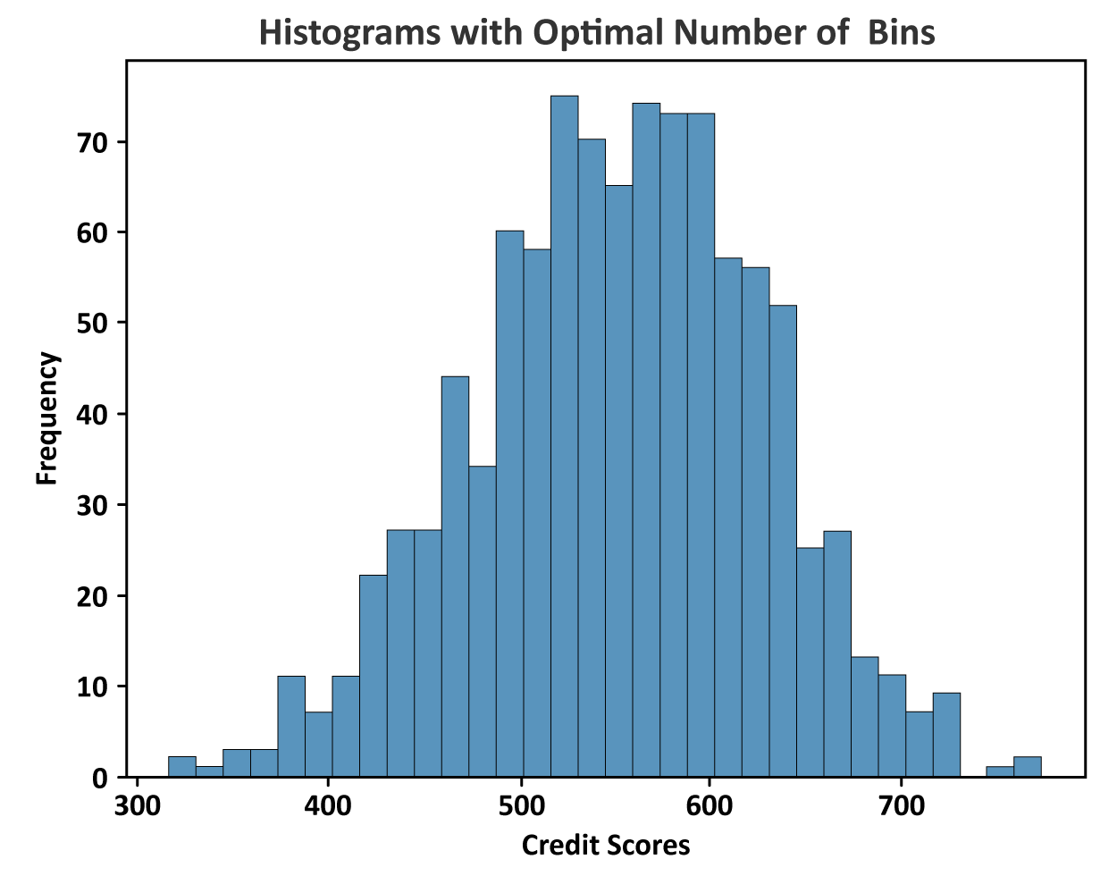
In the credit scores histogram shown previously, suppose the histogram was based on 1,000 credit scores. To find the optimal number of bins we would take the square root of 1,000, which is 31.62 (round up to 32). For the credit scores, an optimal number of bins for the histogram would be 32. The histogram with 32 bins is shown below. This histogram avoids excessive detail or oversimplification. Examining this histogram provides a general sense of the pattern of the credit scores.

Determine the width of the bins. Since a distribution allows you to see every value of the variable, it is important that each observation be captured in each bin. One way to ensure this requirement is to use the following approximation for bin width:

formula to know

Bin Width

This calculation ensures that the entire range of values in the data will be placed into a bin.

hint

In the upcoming example, you will be learning about how to construct a frequency distribution and histogram in Excel. At this point in the course, you should have already created an Excel account and loaded XLMiner Analysis Toolpak. If you have not done so, please refer to Directions to Setup Excel and XLMiner Analysis Toolpak before continuing with the remainder of the lesson.

EXAMPLE

Brenda, the owner of a sporting goods shop, has been collecting sales totals from her last 85 customers. She asks you to help her make sense of these numbers. The table below shows the first 10 of the 85 observations of sales data that Brenda has collected.

Let’s create a frequency distribution for this data and then use the frequency distribution to construct a histogram. You will complete these tasks in Excel.

bin ranges	frequency
30–172	2
173–315	8
316–458	17
459–601	23
602–744	16
745–887	11
888–1,030	6
1,031–1,173	1
1,174–1,316	0
1,317–1,459	1

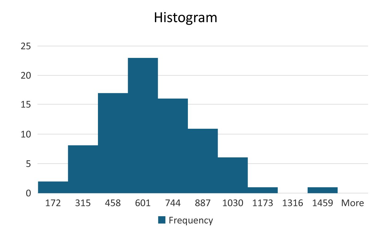
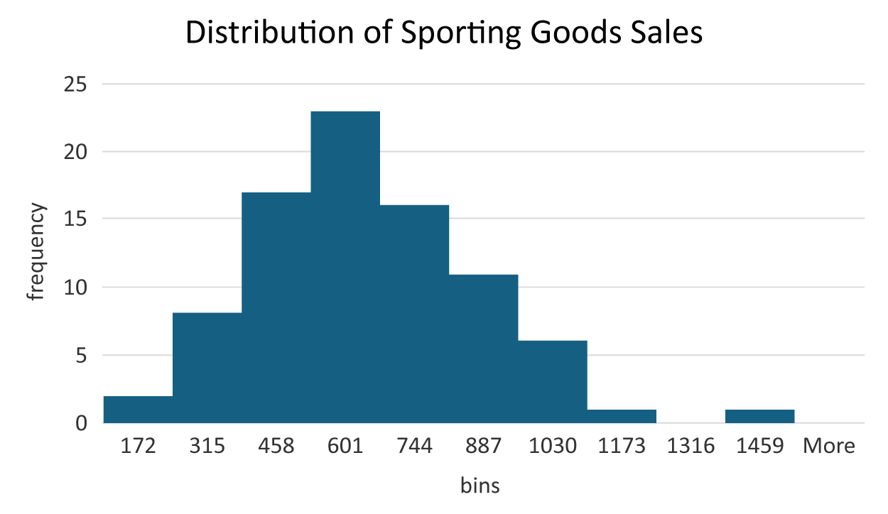
The frequency distribution's creation allows Brenda to observe that most of her sales are between $459 and $601. There are only two sales values between $30 and $172. There is one sale value between $1,317 and $1,459. This could be a potential outlying observation. This one sale value is represented in the bar in the histogram that is to the far right. The histogram allows you to view the frequency distribution of the sales data and detect if there are any potential outliers.

try it

The first thing you will do is construct the number of bins required for the frequency distribution.

Using the square root rule, determine the optimal number of bins for this dataset.

There are 85 observations. which we round up to 10.

try it

The next step is to calculate the bin width. That is, what are the lower and upper bounds for the intervals for each of the bins?

1. Open sporting_goods_sales.xlsx.

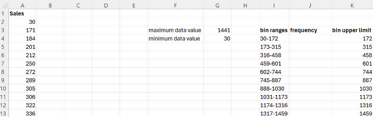
2. Find the maximum and minimum values in a column in Excel by using the =MAX() and =MIN() functions as shown below.



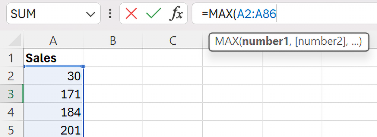
The argument for the MAX() function is the range of data. In this case, the sales data is in column A, from rows 2 to 86 (A2:A86). The colon is used to separate the starting row and the ending row of the data. Do not forget to close the parentheses to end the use of the function. The calculations in Excel are shown below.

maximum data value	=MAX(A2:A86)	1441
minimum data value	=MIN(A2:A86)	30

The maximum data value is 1441 and the minimum data value is 30 so the bin width for this data should be A bin width of about 141 will ensure that 10 bins cover the entire range of values in the dataset.

3. Check your work by comparing your bin width to the one in the example.

watch

Follow along with this video on calculating bin width in Excel.

try it

Construct the frequency distribution and histogram in Excel.

We are going to use the same data as we used above and the calculated minimum and maximum values. So, either continue using the file you were working on, or open this file which contains both the data and the calculated minimum and maximum values: sporting_goods_sales2.xlsx. Perform the following:

1. In the same sheet as your column of data (Sales column), in a cell, create a column named bin ranges that lists the lower and upper values of the bin intervals. Since you know the minimum value is 30, you can use 30 as the lower limit of the first bin.

2. Then, create another column in the cell right beside bin ranges named frequency.

3. Excel uses the upper limits of each bin to count the number of observations in a particular bin, so you need a column that contains the upper limits of each bin. Name this column bin upper limit as shown in the figure below.



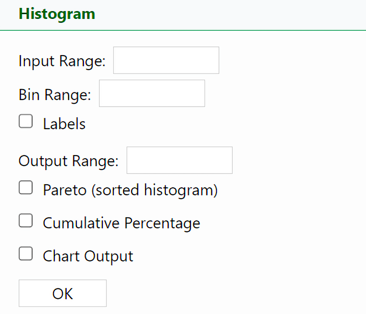
4. Select the Histogram option in the XL Miner Analysis Toolpak. The Histogram dialog box opens.



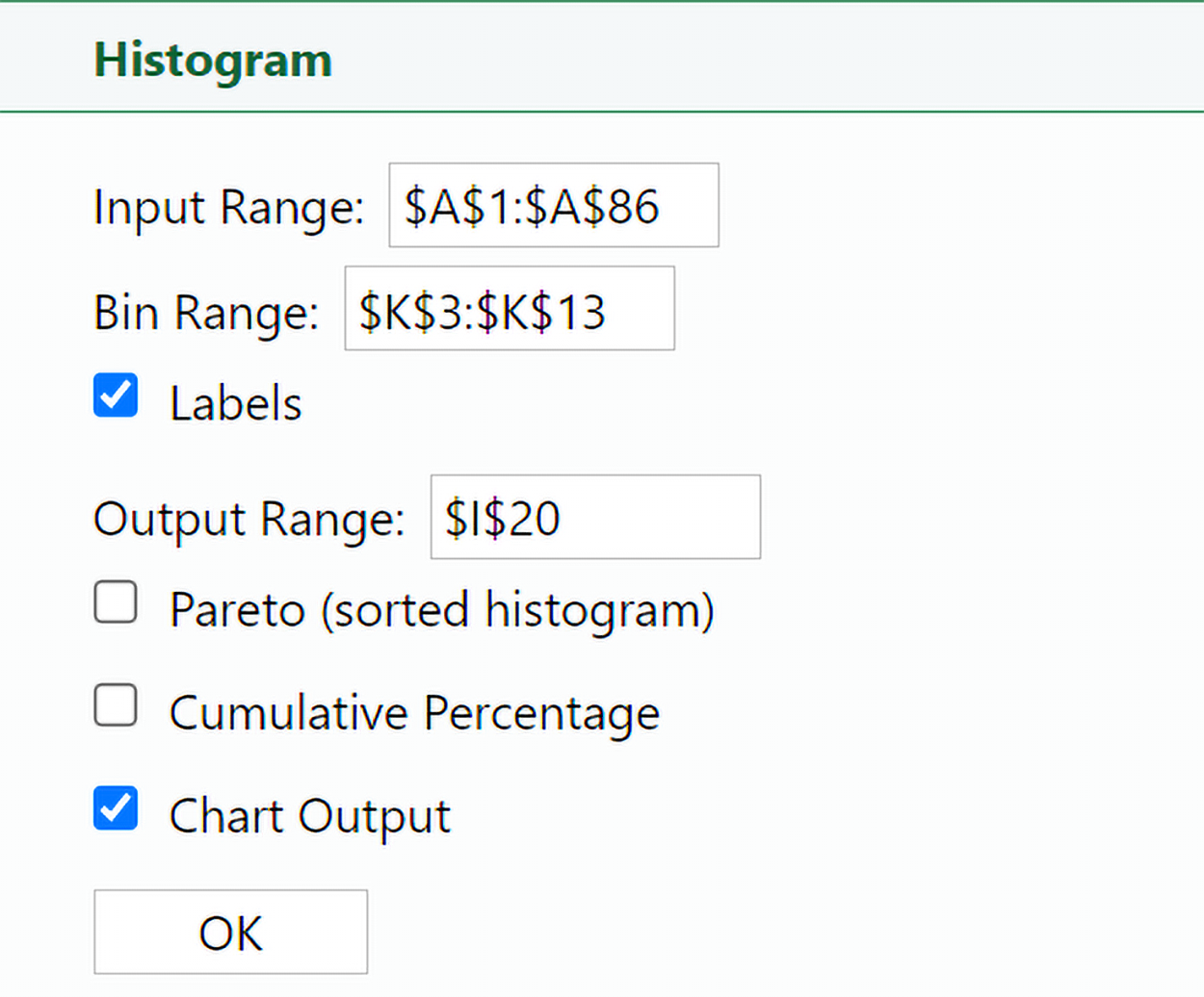
5. Put your cursor in the Input Range box and then use your mouse to select the sales data that are in rows A1 to A86 (include the Sales column label value in row A1). Once you have selected all the data, the Input Range value should now show rows A1 to A86 selected.

Input Range:

$A$1:$A$86

6. Repeat the same process for Bin Range by first putting your cursor in the Bin Range box and then selecting the cells that contain the upper bin limits (cells K3 through K13).

7. Put your cursor in the Output Range box and select any cell in the worksheet. The Output Range box specifies where you want the frequency distribution and histogram to be output. Let’s output the items in the same worksheet as our data.

8. Select the checkbox for Chart Output. This will create the histogram. Then, select the Labels checkbox so that a label will be added to the x-axis (which can be modified). Select OK.



These options produce the following output in Excel.



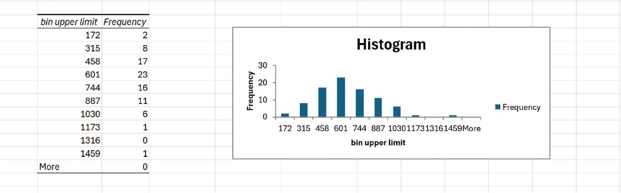
The table to the left is the frequency distribution for the sporting goods sales.

9. Copy the values in the Frequency column to the blank frequency column you created earlier so that you will have a complete frequency distribution as shown in the figure below.



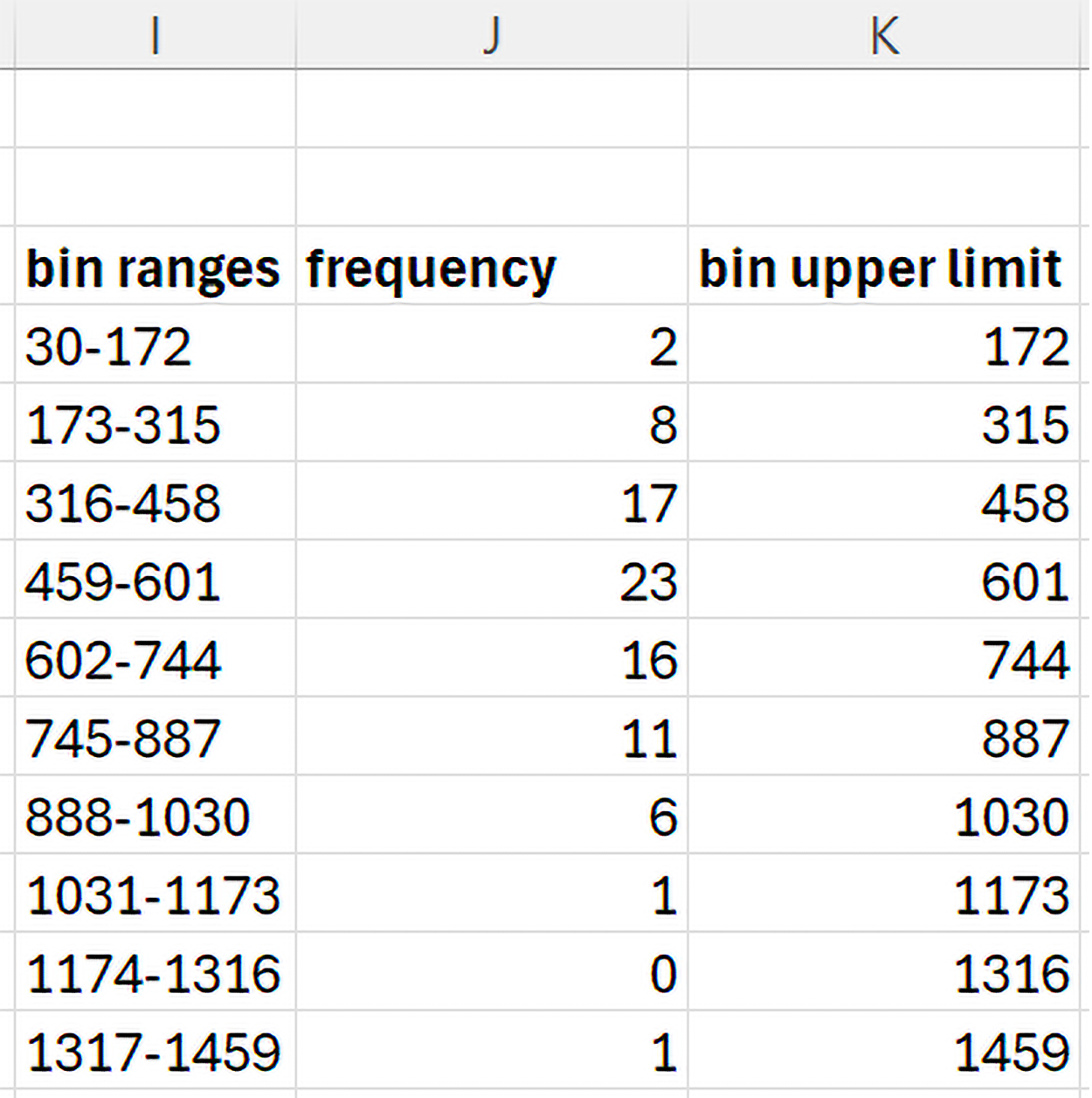
The frequency distribution provides how many sales values are in each bin. For example, two sales were between $30 and $172, eight sales were between $173 and $315, and so on. A frequency distribution can show you where most of the data values lie. For example, most sales amounts were between $459 to $601 because this is the bin with the highest frequency.

10. Check your work by comparing your frequency distribution and histogram to the one in the example.

watch

Follow along with this video on frequency distributions and histograms.

try it

Modify the default histogram in Excel so that the bars touch. Add a title, and label the axes of the histogram.

In a histogram, the bars should touch each other to illustrate that the data is along a numerical axis. This visual continuity helps convey the underlying distribution of a quantitative variable. Notice that the bars in the histogram created by the Analysis Toolpak do not touch by default. You can change the settings of the histogram to make the bars touch each other by performing the following using the same spreadsheet or using this spreadsheet which contains the histogram: sporting_goods_sales3.xlsx

1. Select the Chart menu. Options under the Chart menu allow you to modify the histogram.



2. Select Format (under Chart tab) → Horizontal Axis and set the Gap Width to 0.





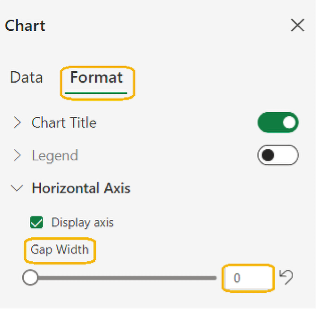
You will now notice the histogram updates so that the bars are touching each other.



To add a chart title and label the axes, perform the following:

3. Select Chart Title (under Chart menu) → Edit Chart Title.



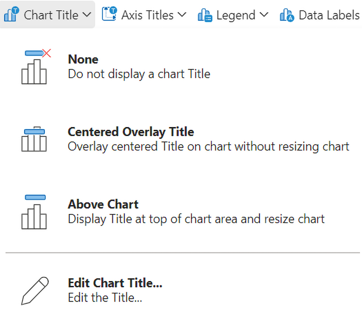
4. Enter "Distribution of Sporting Sales" for the chart title.

5. Select Axis Titles (under Chart menu) → Primary Horizontal Axis Title → Edit Horizontal Axis Title. Enter "bins."

6. Select Axis Titles (under Chart menu) → Primary Vertical Axis Title → Edit Vertical Axis Title. Enter "frequency."

7. In the bottom portion of the histogram, select the legend box named "Frequency" and select Delete to remove the legend.



The final histogram should look like the following:



8. Check your work by comparing your histogram to the one in the example.

watch

Follow along with this video on modifying histograms.

The histogram allows you to visualize the frequency distribution of a quantitative variable. The x-axis represents the bin ranges with the upper limits of each bin being displayed (In a later tutorial, you will be shown how to modify the values displayed in the x-axis). The y-axis is the frequency. The number of observations in each bin (the frequency) is represented by the height of the bars. So, once again, you can see that most sales values fall between $459 and $601 for the sporting goods sales.

You will learn more about histograms and how to interpret them in an upcoming tutorial. For now, it is important to realize that another useful task of a histogram, beyond visualizing a frequency distribution for a quantitative variable, is that they help you detect outliers by looking for bars that are unusually distant from the rest of the distribution. In a previous tutorial, an outlier was defined as a value outside the range of typical values. In examining the histogram, you notice the bar all the way to the right. When you examine the frequency distribution you also notice there is only one data point in the range from $1,317–$1,459 for the sporting goods sales. It is more than likely this is the maximum value in the data, the $1,441 sales value that you identified as the maximum value earlier. This may be a potential outlying value. In the next section, a formal method will be presented to show you how you can formally identify outliers.

term to know

Argument

An input a function needs to produce a result.