Data Types

1. Data Types

Variables can be classified into two data types: quantitative and categorical. A quantitative variable is one that measures/contains values about a numerical quantity or amount. A categorical variable, sometimes called a qualitative variable, classifies people, objects, or units into categories. The table below provides some rules of thumb for differentiating between quantitative and categorical variables.

For quantitative variables, think “numbers.” A quantitative variable tells you how much or how many of some quantity you have, and the average will make sense. Imagine you added up all the values of a quantitative variable column and divided them by the total number of observations you have; would that result (average) make sense?

For a categorical variable, think “categories/levels.” Does the variable classify people, objects, and units into categories? It should not make any sense to take an average of a categorical variable.

EXAMPLE

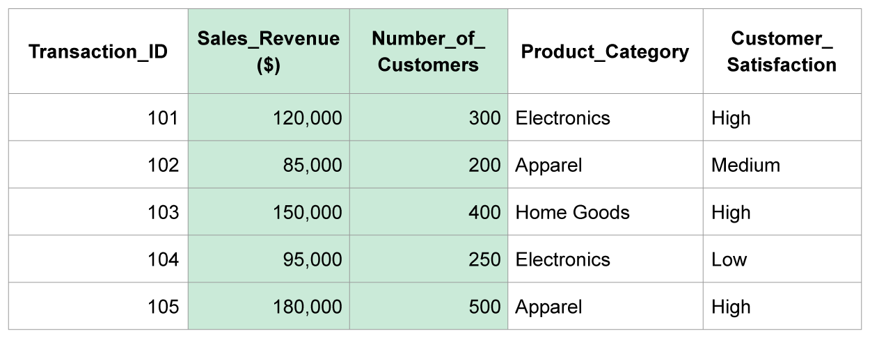
The table below shows some transactional data for a retail company.



The Sales Revenue variable is quantitative because it provides information on how much revenue the company earned. If we added up all the values of Sales Revenue and divided them by five (the total number of observations we have), we would obtain a numerical value of $126,000. This average value makes sense. It represents the average revenue of the company.

Product category is a categorical variable. This variable classifies the items the business sells. Does the average make sense? Well, can you take ‘Electronics’ and add it to ‘Apparel’ and so on, and then, divide that result by five? No, of course not! Even the computation of doing something like that does not make sense. So, the average does not make sense. No arithmetic operations can be performed on a categorical variable.

try it

Consider the remaining variables from the table above:

• Transaction ID
• Number of Customers
• Customer Satisfaction

Classify the variables above as categorical or quantitative.

Transaction ID is categorical because it identifies the transaction, and an average does not make sense.

Number of Customers is quantitative because it indicates “how many” and can be averaged.

Customer Satisfaction is categorical because it describes an aspect of the observation. However, you could imagine if this variable were measured on a scale from 1–10, it could be quantitative.

terms to know

Quantitative Variable

Variables that represent measurable quantities or amounts.

Categorical Variable

Represents labels for people, objects, or units.

Qualitative Variable

Another term used to describe a categorical variable.

1a. Measurement Levels for Quantitative Data

There are three measurement levels for quantitative data; continuous, ratio, and discrete. A measurement level describes the scale of the variable. The measurement level lets you know what type of mathematical operation is appropriate for the variable. For example, can an average value be computed, or is another measure more appropriate? A continuous measurement level means the variable's value can take on any value in an interval. Continuous measurement levels can contain decimals. A ratio measurement level contains all the characteristics of a continuous measurement level with the additional aspect of a true zero point. Meaning zero represents the absence of the value. For example, a salary of $0 represents no income. Zero inventory represents no items. A profit margin of 0% means no profit. Contrast the meaning of a zero value for a continuous measurement level. For example, temperature that is measured in Fahrenheit or Celsius degrees. Zero degrees Fahrenheit does not mean “no temperature;” it is just a reference point. A discrete measurement level means the variable’s value cannot take on a value in an interval. Discrete measurement levels are integers; they cannot take decimal values.

key concept

Measurement level determines the types of analyses and operations you can perform with a particular variable. It’s important to identify the level when collecting data so you can plan your analytical methods.

Returning to the retail data shown in the table below, Sales Revenue has a continuous measurement level because sales can take on a value in an interval. For example, the company could have earned $50,000.50. This is a viable value for Sales Revenue. The Number of Customers has a discrete measurement level because the company cannot have 300.5 customers. You cannot viably have half a person. The Number of Customers variable is measured in integers only and cannot take on a value in an interval.

try it

Consider the following variables:

• Interest rates
• Inventory numbers
• Customer satisfaction (star rating)

Classify these variables as discrete or continuous.

Interest rates are continuous because they can take on any value in an interval.

Inventory is discrete because you generally can’t have a non-integer quantity of goods.

Customer star rating is discrete because users can choose only 1, 2, 3, 4, or 5 stars.

terms to know

Measurement Level

Classification of data based on characteristics that determine which analytical techniques are possible.

Continuous Measurement Level

Any numeric value in a range, including decimals, is used to measure a quantitative variable.

Ratio Measurement Level

A continuous measurement level in which the value zero represents the absence of the quantity.

Discrete Measurement Level

Whole numbers, which are used to measure a quantitative variable.

1b. Measurement Levels for Categorical Data

There are two measurement levels for categorical data; nominal and ordinal. A nominal measurement level means the categories have no natural order to them. Whereas, at an ordinal measurement level, the categories do have a natural order to them. Using the retail data again, you can see in the table below that the variable Product Category is nominal. The categories "Electronics," "Apparel," etc. are simply labels for the items sold, and there is not one category that is "naturally higher" than another. Electronics is not higher or better than Apparel.

Customer satisfaction is an ordinal variable. An ordinal variable refers to a type of data where the categories have a natural order or ranking, but the distances between the categories are not meaningful. In the case of Customer Satisfaction, this means that we can order responses (e.g., “very dissatisfied,” “neutral,” “very satisfied”) from lowest to highest. Ordinal measurement levels are common in surveys and rating scales, where the order matters.

try it

Emil is gathering primary data by surveying employees at different levels about job satisfaction at his company.

What types of questions might Emil ask to gather nominal and ordinal data?

Question Type	Nominal	Ordinal
Employee Information	Job Title: "Software Engineer," "Product Manager," "Data Analyst"	Job Level: (Junior < Mid-level < Senior < Executive)
Job Feedback	Feedback Category: "Work/Life Balance," "Compensation," "Benefits"	Satisfaction Level (Very Dissatisfied < Dissatisfied < Neutral < Satisfied < Very Satisfied)
Work Location	Work Arrangement: "On-site," "Hybrid," "Remote"	Commute Difficulty: (Easy < Moderate < Difficult < Very Difficult)

terms to know

Nominal Measurement Level

Label used to classify categorical variables without assigning rank-order values to them.

Ordinal Measurement Level

Label used to classify categorical variables where a rank-order of the labels is assigned.

1c. Comparing Measurement Levels

Knowing your data type and the associated measurement levels is important because it impacts the types and number of analytical methods you can apply. You can use more analytical methods with quantitative data than you can with categorical data.

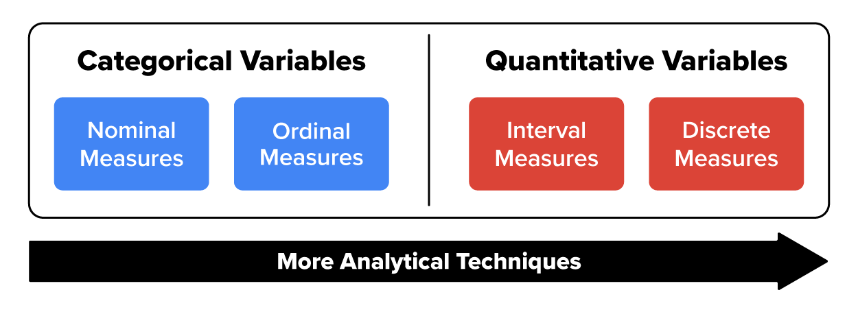
The table below shows the different types of analytical methods that can be used based on the measurement level of the variables. For interval and discrete measurement level data, you have more analytical methods at your disposal.

1d. Importance of Data Type and Measurement Levels in Business Data Analytics

By recognizing the data type and its measurement level, you can choose the appropriate statistical technique, create appropriate visualizations, and draw meaningful insights from your data. If you do not recognize the appropriate data type and measurement level, the results from your analysis will have unintended consequences. Consider the scenario below.

IN CONTEXT

You are working for an online retailer. The company wants to conduct a customer satisfaction survey about a new fast checkout process on their mobile app. The company collects feedback on a scale from 1 (very dissatisfied) to 5 (very satisfied). The customer feedback data is ordinal because the scale of the data (1 to 5) has an order to the values. Suppose you have 100 customer responses.

• 50 customers provide a rating of 5 (very satisfied).
• 50 customers provide a rating of 1 (very dissatisfied).

You treat the customer satisfaction scores as continuous data and take the average of the values as follows:

You report an average of 3 but realize this does not make sense because it implies a moderate satisfaction level, which contradicts the extreme ratings (1 and 5) given by customers. Managers might wrongly assume everything is fine based on the neutral sentiment. However, the average does not reflect the large number of customers who are very dissatisfied.

The average calculation provided is not correct because the average ignores the ordinal nature of the data. The difference between each rating level is not uniform. Going from “neutral” (3) to “satisfied” (4) may not represent the same change in satisfaction as going from “dissatisfied” (2) to “neutral” (3).

A better approach to understanding this data would be to construct a visualization like a column chart shown below that shows the distribution of the customer ratings.



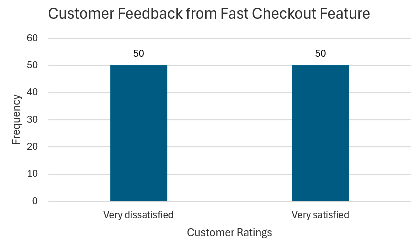
You will learn how to create a column chart like this one in the next tutorial. Understanding data type and measurement level ensures meaningful analysis and prevents misleading conclusions!