Use Sophia to knock out your gen-ed requirements quickly and affordably. Learn more
×

Creating a Full Monte Carlo Simulation and Scenario Analysis

Author: Sophia

what's covered
In this lesson, you will learn how to extend your knowledge from single-instance Monte Carlo simulations to full Monte Carlo simulations and evaluate the simulation results. Specifically, this lesson will cover:

Table of Contents

1. Full Monte Carlo Simulation

In the previous lesson, you were introduced to single-instance Monte Carlo simulation, where the simulation was run only once to provide a quick estimate of the outcome based on one set of random samples. Now, you will take this a step further by running a full Monte Carlo simulation. This involves running the simulation multiple times to capture the variability and range of possible outcomes, providing a more comprehensive understanding of the potential scenarios.

1a. Comparing a Full Monte Carlo Simulation to a Single-Instance Monte Carlo Simulation

For each step, a comparison to the single-instance Monte Carlo simulation is provided.

  1. Define the Problem. The same as in a single-instance simulation, clearly define the problem you want to solve. Identify the key random variables and the outcomes you are interested in estimating.
  2. Determine the Probability Distribution. The same as in a single-instance simulation, identify the probability distributions for the random variables.
  3. Generate Random Samples. The same as in a single-instance simulation, use random sampling to generate many possible values for the random variables based on their probability distributions.
  4. Perform the Simulations. Unlike the single-instance simulation, run the simulation multiple times (for example, 1,000 simulations). For each simulation, generate a new set of random samples and calculate the outcomes. This captures the variability and range of possible outcomes.
  5. Analyze the Results. Unlike the single-instance simulation, Analyze the results of all the simulations to understand the distribution of the outcomes. Calculate summary statistics (mean, median, standard deviation) for the entire set of simulated outcomes (not just from one simulation) and visualize the results using histograms or other charts.
  6. Interpret the Results (turn the results into insights). Interpret the insights gained from the multiple simulations.
The table below highlights the key differences between a single-instance Monte Carlo simulation and a full Monte Carlo simulation.

Aspect Single-Instance Monte Carlo Simulation Full Monte Carlo Simulation
Number of Simulations Runs the simulation only once. Runs the simulation multiple times (1,000 simulations).
Capturing Variability Provides a quick estimate based on one set of random samples, which may not fully capture variability and uncertainty. Captures the variability and range of possible outcomes by running multiple simulations, providing a more comprehensive understanding.
Analyzing Results Analyzes the result from one simulation. Analyzes the results from multiple simulations, providing a more detailed and accurate analysis.
Interpretation and Insights Offers preliminary insights based on one set of data. Provides more thorough and reliable insights by considering the variability across multiple simulations, making it better suited for informed decision-making.

1b. Full Monte Carlo Simulation in Python

Let's construct a full Monte Carlo simulation model in Python using an example that you are familiar with from the previous tutorial.

EXAMPLE

GizmoHub is a small e-commerce business that sells the latest tech gadgets, including smartphones, tablets, and accessories. The store has been operating for a year, and the management is keen to understand its revenue patterns better to make informed decisions about inventory, marketing, and financial planning.

The management at GizmoHub has noticed that their daily revenue varies significantly due to factors like promotions, holidays, and market trends. They want to estimate the average monthly revenue to plan their budget and set realistic sales targets for the upcoming year. However, the variability in daily revenue makes it challenging to predict monthly revenue accurately.

You are a business data analyst at GizmoHub. You decide to construct a full Monte Carlo simulation with 1,000 simulations to estimate the average monthly revenue. This approach provides a more thorough and reliable estimate of potential monthly revenues for GizmoHub.

The code below installs and imports the necessary libraries and performs a full Monte Carlo simulation. This code runs the Monte Carlo simulation 1000 times, generating a range of possible monthly revenues. It then calculates and prints the average, median, and standard deviation of the simulated monthly revenues, and visualizes the distribution. The output from the Monte Carlo simulation is also provided.

It is important to note that the code that sets up the environment by importing pyodide_http for internet requests and installing essential packages (numpy and matplotlib) using micropip is missing from the screenshot below but is required before you run the code shown in the screenshot.


Let’s break down the code to understand how you can implement the Monte Carlo simulation.

Step 1: Define the Problem

GizmoHub, a small e-commerce business specializing in tech gadgets, wants to better understand their revenue patterns to make informed decisions about inventory, marketing, and financial planning. The management has observed significant variability in daily revenue due to factors such as promotions, holidays, and market trends. To plan their budget and set realistic sales targets for the upcoming year, they need to estimate the average monthly revenue.

In this context, the random variable is the daily revenue, which can vary between $200 and $1,000. The outcome of interest is the average monthly revenue, which will help GizmoHub account for the variability in daily revenue and provide a range of possible outcomes for better decision-making.

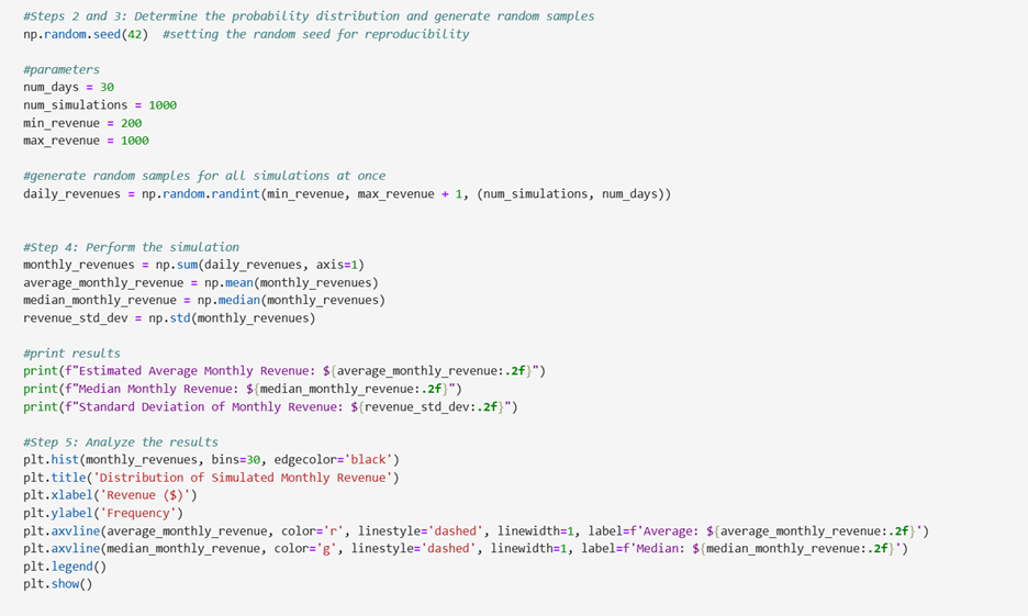
Steps 2 and 3: Determine the Probability Distribution and Generate Random Samples
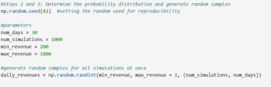


np.random.seed(42)
  • This line sets the random seed to 42, ensuring that the random numbers generated are the same each time the code is run.
num_days = 30
num_simulations = 1000
min_revenue = 200
max_revenue = 1000
  • The lines above define the parameters of the Monte Carlo simulation. They help set up the environment in which the simulation runs and determine the range of the random variables involved.
daily_revenues = np.random.randint(min_revenue, max_revenue + 1, (num_simulations, num_days))
  • This line generates random daily revenues for all simulations at once. It creates a 2D array where each row represents a simulation, and each column represents a day. The values are randomly chosen between $200 and $1,000.
Step 4: Perform the Simulations


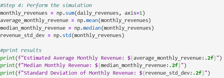
monthly_revenues = np.sum(daily_revenues, axis=1)
  • This line calculates the monthly revenue for each simulation by summing the daily revenues. The axis=1 argument ensures that the sum is calculated across the columns (days) for each row (simulation).
average_monthly_revenue = np.mean(monthly_revenues)
median_monthly_revenue = np.median(monthly_revenues)
revenue_std_dev = np.std(monthly_revenues)
  • average_monthly_revenue: Calculates the average monthly revenue across all simulations.
  • median_monthly_revenue: Calculates the median monthly revenue across all simulations.
  • revenue_std_dev: Calculates the standard deviation of the monthly revenues, indicating the variability.
print(f"Estimated Average Monthly Revenue: ${average_monthly_revenue:.2f}")
print(f"Median Monthly Revenue: ${median_monthly_revenue:.2f}")
print(f"Standard Deviation of Monthly Revenue: ${revenue_std_dev:.2f}")
  • These lines print the calculated statistics, providing an estimate of the average, median, and standard deviation of the monthly revenues.
Step 5: Analyze the Results


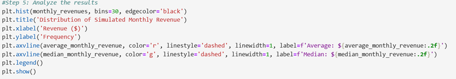
plt.hist(monthly_revenues, bins=30, edgecolor='black')
plt.title('Distribution of Simulated Monthly Revenue')
plt.xlabel('Revenue ($)')
plt.ylabel('Frequency')
plt.axvline(average_monthly_revenue, color='r', linestyle='dashed', linewidth=1, label=f'Average: ${average_monthly_revenue:.2f}')
plt.axvline(median_monthly_revenue, color='g', linestyle='dashed', linewidth=1, label=f'Median: ${median_monthly_revenue:.2f}')
plt.legend()
plt.show()
  • plt.hist: Creates a histogram to visualize the distribution of the simulated monthly revenues.
  • plt.title: Sets the title of the histogram.
  • plt.xlabel: Labels the x-axis as "Revenue ($)."
  • plt.ylabel: Labels the y-axis as "Frequency."
  • plt.axvline: Adds vertical dashed lines to indicate the average and median monthly revenues on the histogram.
  • plt.legend: Adds a legend to the histogram.
  • plt.show: Displays the histogram.
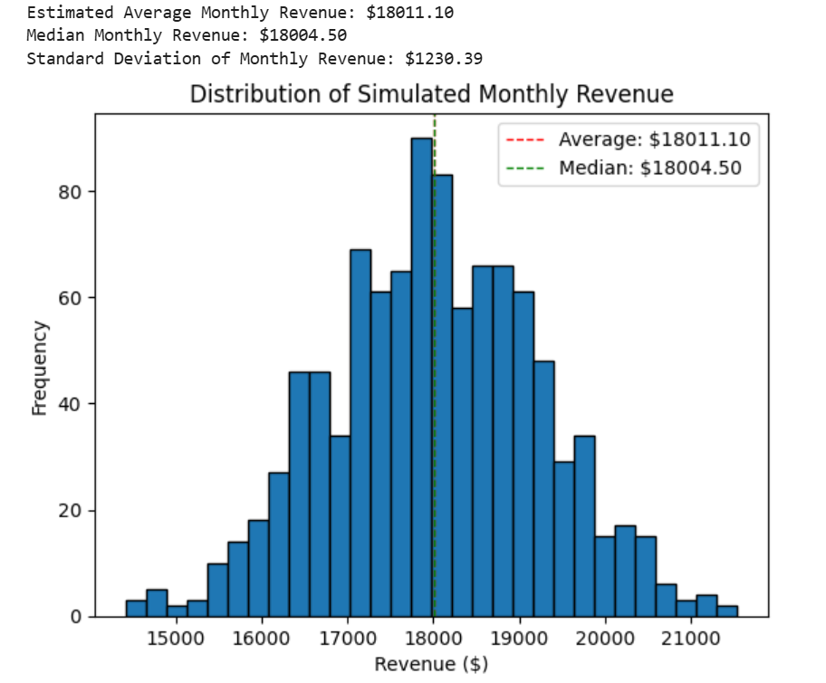
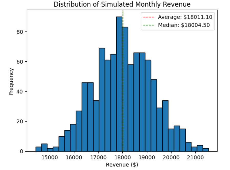
The histogram visualizes the distribution of the simulated monthly revenues from the full Monte Carlo simulation using 1,000 simulated daily revenue values. Here’s what it shows:

  • Frequency Distribution: The x-axis represents the range of monthly revenues, while the y-axis represents the frequency (how often each revenue range occurs across the simulations).
  • Average Monthly Revenue: A red dashed line indicates the average monthly revenue across all simulations.
  • Median Monthly Revenue: A green dashed line indicates the median monthly revenue across all simulations.


Step 6: Interpret the Results

Interpretation of the Average and Median Revenue Values from the Full Monte Carlo Simulation:

Average Monthly Revenue

The average monthly revenue (mean) is calculated by summing all the simulated monthly revenues and dividing by the number of simulations. In the context of GizmoHub, the average monthly revenue provides an estimate of what the typical monthly revenue might be, considering the variability in daily revenues due to factors like promotions, holidays, and market trends.

  • Context: For GizmoHub, the average monthly revenue helps the management understand the expected revenue over a month, considering the range of possible daily revenues. This figure is useful for budgeting, financial planning, and setting sales targets.
Median Monthly Revenue

The median monthly revenue is the middle value of the simulated monthly revenues when they are sorted in ascending order. It represents the point at which half of the simulated monthly revenues are below and half are above.

  • Context: For GizmoHub, the median monthly revenue provides an estimate that is less affected by extreme values (outliers) compared to the average. This is particularly useful if there are occasional very high or very low daily revenues that could skew the average. The median gives a more robust measure of the central tendency of the monthly revenues.
Practical Implications

  • Budgeting and Financial Planning: Both the average and median monthly revenues help GizmoHub set realistic budgets and financial plans. The average gives a general expectation, while the median provides a more stable estimate.
  • Sales Targets: Understanding both metrics allows GizmoHub to set achievable sales targets. The average helps in setting optimistic targets, while the median ensures that targets are realistic and not overly influenced by outliers.
  • Risk Management: By considering both the average and median, GizmoHub can better manage financial risks. The average helps in understanding the overall expected revenue, while the median provides a safeguard against extreme variations.
In summary, the average monthly revenue gives a general expectation of monthly revenue, while the median monthly revenue provides a more stable estimate that is less influenced by outliers. Both metrics are crucial for making informed decisions about inventory, marketing, and financial planning at GizmoHub.

Interpretation of the Standard Deviation from the Full Monte Carlo Simulation:

The standard deviation of $1,230.39 in the context of GizmoHub's Monte Carlo simulation represents the variability or dispersion in the simulated monthly revenues. This value provides insight into how much the monthly revenues are expected to fluctuate around the average monthly revenue.

Practical Implications

  • Revenue Fluctuations: The standard deviation indicates that the monthly revenues can vary by approximately $1,230.39 from the average monthly revenue. This helps GizmoHub understand the extent of revenue fluctuations they might experience, due to factors like promotions, holidays, and market trends.
  • Risk Management: By knowing the standard deviation, GizmoHub can better prepare for months with lower-than-average revenues. This information is crucial for managing financial risks and ensuring that the business can sustain operations even during less profitable months.
  • Inventory and Staffing Decisions: The variability in monthly revenues can impact inventory and staffing needs. For example, during months with higher revenues, GizmoHub might need more inventory and staff to handle increased demand. Conversely, during months with lower revenues, they might need to adjust inventory orders and staffing levels to avoid excess costs.
In summary, the standard deviation of $1,230.39 provides GizmoHub with valuable insights into the variability of their monthly revenues. This information is essential for making informed decisions about inventory, staffing, and risk management, ultimately helping the business operate more efficiently and sustainably.


Now, try constructing your own full Monte Carlo simulation!

try it
FreshBites Bakery is a small bakery that specializes in delivering fresh, homemade baked goods, including cakes, cookies, and pastries. The bakery has been operating for a year, and the management wants to understand their daily order patterns better to make informed decisions about inventory, staffing, and operations.

The management at FreshBites has noticed that their daily orders vary significantly due to factors like promotions, holidays, and customer preferences. They want to estimate the average monthly orders to plan their operations and set realistic targets for the upcoming year. However, the variability in daily orders makes it challenging to predict monthly orders accurately.

You are a business data analyst at FreshBites. You want to use a full Monte Carlo simulation to estimate the average monthly orders. This approach will help account for the variability in daily orders and provide a range of possible outcomes.

Construct a full Monte Carlo simulation with 1,000 simulations to estimate the average monthly orders for FreshBites Bakery. Follow the requirements below:

  • The daily orders can vary between 20 and 100 orders daily. Assume the daily orders follow a uniform distribution.
  • Use a random seed value of 42 so that your results will be reproducible.
  • Generate random samples for 1000 simulations, each representing a month of daily orders.
  • Calculate the average monthly orders from the simulated data.
  • Construct a histogram to visualize the distribution of simulated monthly orders.
Using the Monte Carlo simulation you constructed with the above requirements, answer the following questions:

  1. What is the estimated average monthly orders for FreshBites Bakery?
  2. What is the median monthly orders?
  3. What is the standard deviation of the monthly orders?
  4. How does the histogram help in understanding the variability in monthly orders?
Solution:

The image below provides the code that meets the requirements of the Monte Carlo simulation.


  1. Approximately 1,798.
  2. 1,806
  3. Approximately 130.
  4. The histogram provides a visual representation of the distribution of simulated monthly orders for FreshBites Bakery. Here’s how it helps in understanding the variability:

    Frequency Distribution: The histogram shows how frequently different ranges of monthly orders occur across the 1000 simulations. This helps FreshBites see which order ranges are most common and which are less likely.

    Spread of Data: The overall spread of the data shows the variability in monthly orders. A wider spread indicates more variability, while a narrower spread indicates less variability. This helps FreshBites understand how much the monthly orders can fluctuate.

    Outliers and Extremes: The histogram can also highlight any outliers or extreme values in the data. If there are bars far away from the central cluster, it indicates that there are some months with significantly higher or lower orders than the average.

    Shape of Distribution: The shape of the histogram (for example, symmetric, skewed) provides insights into the distribution of monthly orders. For example, a symmetric histogram suggests that the orders are evenly distributed around the average, while a skewed histogram indicates that there are more months with orders on one side of the average.

watch
Follow along with this video on how to use Python to construct a full Monte Carlo simulation to estimate average monthly orders.


2. Scenario Analysis

Scenario analysis is a tool used to evaluate the potential outcomes of different decisions under uncertainty. For example, by incorporating Monte Carlo simulations, GizmoHub can model a wide range of possible scenarios for its wearable devices and app features. This approach generates random variables and runs numerous simulations to provide a comprehensive view of potential risks and rewards. For instance, GizmoHub can use Monte Carlo simulations to predict the impact of new features on user engagement or to assess the reliability of location tracking under various conditions. This method enables GizmoHub to make more informed decisions, enhancing strategic planning and risk management to ensure the safety and satisfaction of its users.

term to know
Scenario Analysis
A process used to evaluate and understand the potential outcomes of different decisions or actions under various conditions in a Monte Carlo simulation.

2a. Implementing the Scenario Analysis

Implementing a scenario analysis involves several key steps to ensure a thorough and effective evaluation of potential outcomes. Here’s a structured approach to guide you through the process that uses the familiar GizmoHub example:

  1. Define Objectives: GizmoHub aims to evaluate the potential impact of introducing a new feature in its wearable devices that enhances location tracking accuracy.
  2. Identify Key Variables: Key variables include user engagement rates, device battery life, data accuracy, and market adoption rates.
  3. Gather Data: GizmoHub collects historical data on user engagement, battery performance, and market trends from previous feature launches and industry reports.
  4. Develop Scenarios: GizmoHub creates scenarios, such as:
    1. Best-Case: High user engagement, minimal impact on battery life, and rapid market adoption.
    2. Worst-Case: Low user engagement, significant battery drain, and slow market adoption.
    3. Moderate-Case: Average user engagement, manageable battery impact, and steady market adoption.
  5. Run Monte Carlo Simulations: GizmoHub uses Monte Carlo simulations to model these scenarios by generating random values for the key variables based on their probability distributions. Thousands of simulations are run to produce a range of possible outcomes.
  6. Analyze Results: The results show the distribution of potential outcomes, highlighting the likelihood of different levels of user engagement, battery performance, and market adoption.
  7. Make Informed Decisions: GizmoHub uses these insights to decide whether to proceed with the feature launch, adjust the feature to optimize battery life, or implement additional marketing strategies to boost adoption.
  8. Monitor and Adjust: Post-launch, GizmoHub continuously monitors user feedback and performance data, adjusting the feature and scenarios as new information becomes available.

2b. Insights from the Scenario Analysis

The insights derived from scenario analysis are invaluable for strategic decision-making and risk management. By examining the range of possible outcomes generated through Monte Carlo simulations, organizations can gain a deeper understanding of the potential impacts of their decisions. Here are some key insights that can be obtained for the scenario analysis that GizmoHub implemented.

  1. Risk Identification: The analysis identifies the risk of significant battery drain, which could negatively impact user satisfaction.
  2. Opportunity Recognition: The best-case scenario reveals an opportunity to significantly increase user engagement if the feature performs well.
  3. Sensitivity Analysis: The analysis shows that battery life is the most sensitive variable, indicating that even small changes in battery performance can significantly impact user satisfaction.
  4. Probability Distributions: The simulations provide a probability distribution of user engagement levels, helping GizmoHub understand the most likely outcomes.
  5. Strategic Planning: Insights from the analysis inform GizmoHub's strategic planning, leading to the decision to enhance battery optimization before the feature launch.
  6. Resource Allocation: GizmoHub allocates additional resources to battery optimization and user education to mitigate the identified risks.
  7. Performance Metrics: The analysis sets realistic performance metrics for user engagement and battery life, helping GizmoHub track progress and make necessary adjustments.
By applying scenario analysis and Monte Carlo simulations, GizmoHub can make data-driven decisions that enhance the success of new features and improve overall user satisfaction.

summary
In this lesson, you were guided through extending your knowledge from single-instance Monte Carlo simulations to full Monte Carlo simulations and evaluating the results. You learned how to run multiple simulations to capture the variability and range of possible outcomes, comparing full Monte Carlo simulations to single-instance ones, and implementing these simulations in Python. You continued with the example of a small e-commerce business, gaining insights into how to estimate average monthly revenue and make informed decisions about inventory and financial planning, based on the simulation results. Additionally, you explored scenario analysis to identify risks, recognize opportunities, and provide the e-commerce business with a methodology to make data-driven decisions in the presence of uncertainty.

Source: THIS TUTORIAL WAS AUTHORED BY SOPHIA LEARNING. PLEASE SEE OUR TERMS OF USE.

Terms to Know
Scenario Analysis

A process used to evaluate and understand the potential outcomes of different decisions or actions under various conditions in a Monte Carlo simulation.