Table of Contents |
Statistics are used regularly in our everyday lives. For example, you may hear information presented in the news about political polls or crime rate increases, or you may determine the likelihood of winning the lottery or getting into a car accident. For this lesson, we’ll ease into statistics by looking at the Counting Principle which explores the possibilities of certain events or things happening. If you have a result in mind that you’d like to achieve, and this result is purely up to chance, you can determine the chances of achieving this result with the fundamental counting principle.
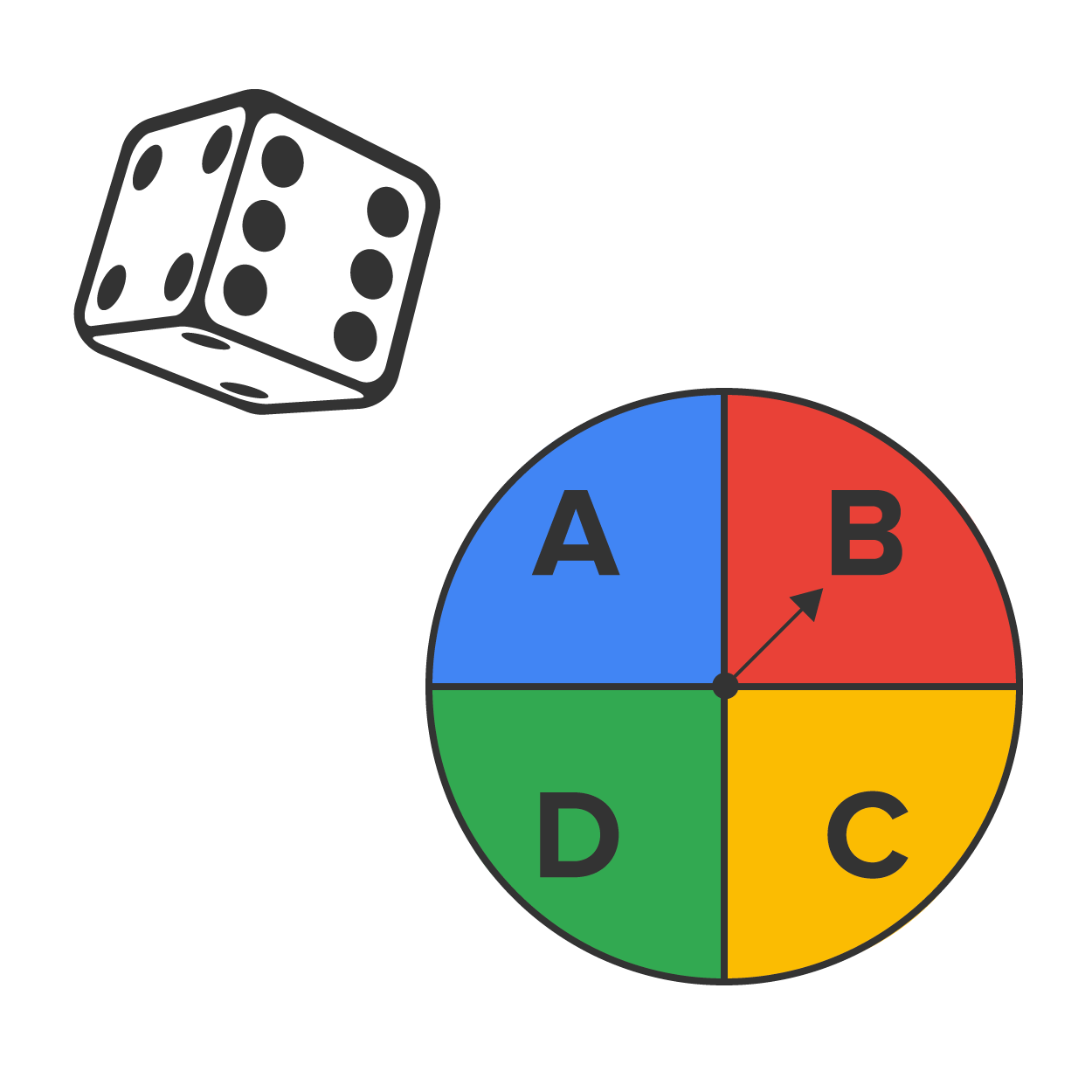 Consider a chance experiment where you roll a standard die and spin this spinner to choose a letter. Each of these spinning sections are equally likely, because there are four equal sections. How many different outcomes of this experiment are possible given that we are choosing rolling one number from the die and selecting one letter from the spinner?
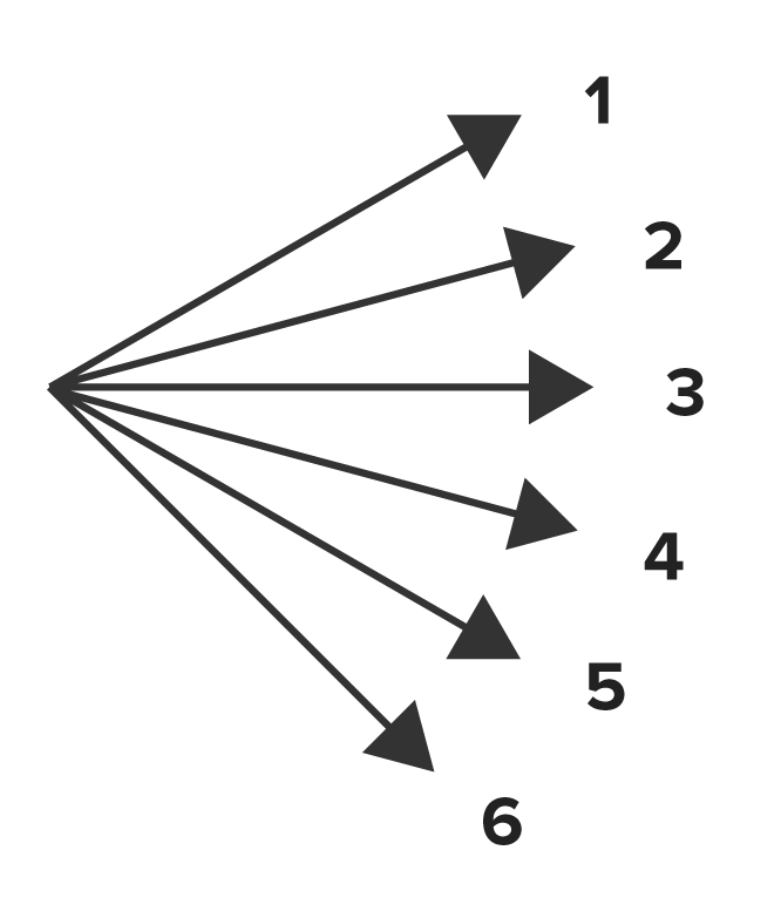
One way to visualize this is with something we call a tree diagram. A tree diagram is a way to visually draw out each of the possibilities. To start, we're going to enumerate all the possible outcomes that could happen from the first chance experiment, which is rolling the die. So, we're going to make a tree with six possibilities for the die: 1, 2, 3, 4, 5, and 6.
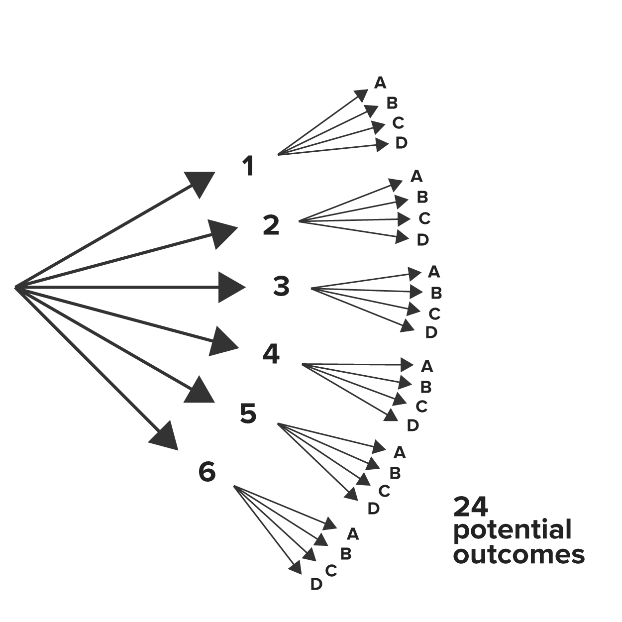
Next in the tree are all the possibilities for the spinner, for each possibility for the die. For instance, if a 1 is rolled, the spinner might spin A, B, C, or D. If a 2 is rolled, the spinner might land on A, B, C, or D, etc. Each outcome represents a different path: one path is 1, C, for example. Another path is 1, D, and so forth. What you end up seeing are 24 different outcomes.
There are six branches for the die, each of which has four outcomes for the spinner. So it's like calculating 6 times 4.
In fact, that's what the fundamental counting principle says. It says if you do two chance experiments, A and B, then experiment A has m potential outcomes and experiment B has n potential outcomes. It follows, then, that there are m times n potential outcomes when experiments A and B are performed together.
The fundamental counting principle can actually extend beyond just two experiments. It can extend to three, four, five, or however many experiments are being conducted together, by simply multiplying the number of potential outcomes for each consecutive experiment. In the example above, there were 6 outcomes for the die and 4 outcomes for the spinner, so there were 6 times 4, or 24 potential outcomes.
IN CONTEXT
A family is going to have three children. How many different orderings of children are there in terms of boys and girls?
The first child could be a boy or a girl. If you start with a boy, you could have another boy, and the third child could be a girl. Another outcome is that you could have three boys.
If you start with a girl, the second and third child could both be boys. Another outcome could be that you have two girls, then have a boy.
As you can see, there are many different outcomes. To find all possible outcomes, you can create a tree diagram.
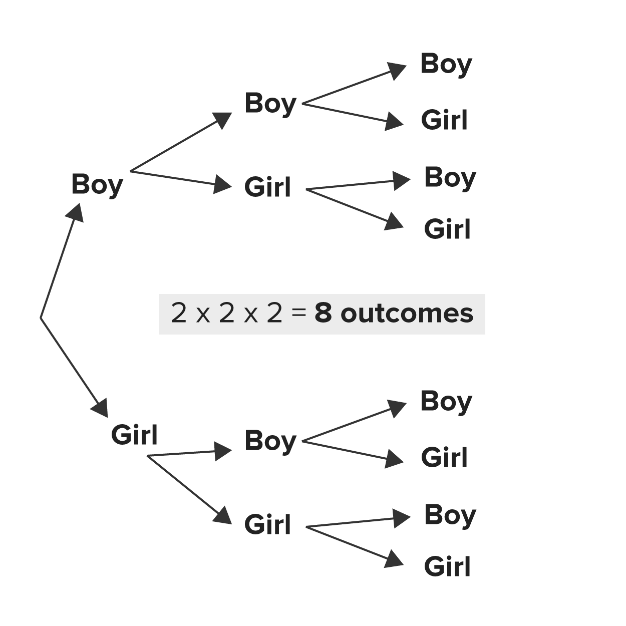
Looking at all the tree diagram branches here, you can see there are eight possible outcomes.
An easier way to do it would be to use the Fundamental Counting Principle. For the first child, there are two options; for the second child, two options; and for the third child, two options.
So, 2 times 2 times 2 equals 8 outcomes. The tree diagram isn't really necessary. The number of choices for each of the children multiplied by each outcome for the children is what is needed.
IN CONTEXT
Your closet consists of 5 shirts, 3 pants, 1 skirt, and 2 blazers. For work, you need to wear a shirt, some type of bottom (skirt or pants) and a blazer. How many different outfits can you create for work?
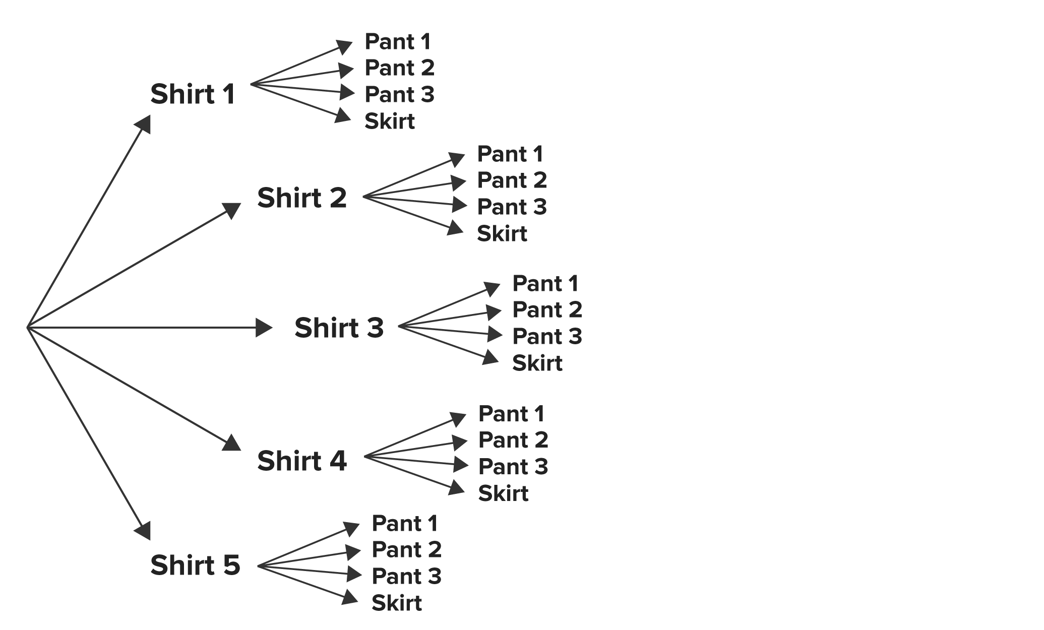
First, create your tree diagram. It does not matter which of the items of clothing you start with, but it is recommended that you start with the largest value with your first “branch” so your later branches aren’t too busy and little to count.

Next, we can account for our type of bottoms. Because you wouldn’t wear a pair of pants and a skirt, we have a total of 4 choices of bottoms to choose from, as seen here:
For each of these top and bottom clothing choices, we can now pair it with one of our two blazers as seen here:
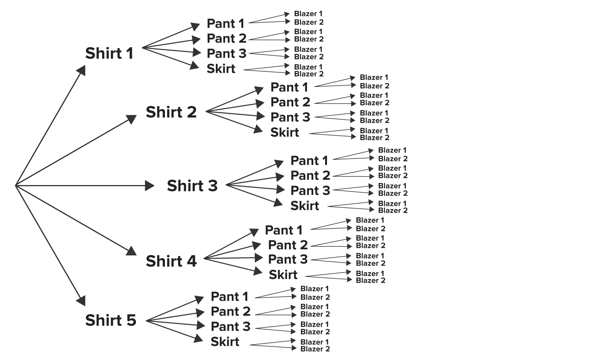
As we can see, we have a total of 40 unique outfits that can be created from our clothing choices. Granted, some of these pieces of clothing may not match well, but each is still a potential wardrobe option.
Meanwhile, drawing this tree could have taken you quite a bit of time. How could we accomplish determining how many unique outfits could be created without drawing it? Remember, we can simply multiply each of the possibilities together:
To recap, 4 bottoms times 5 tops times 2 blazers = 40 unique outfits.
Results Driven: Apply Your Skill |
 ) potential outcomes when A and B are done together.
Source: THIS TUTORIAL WAS AUTHORED BY SOPHIA LEARNING. PLEASE SEE OUR TERMS OF USE.