Economies of scale is generally a long run concept.
The firm can alter its factory size and therefore really affect their scale of operation.
EXAMPLE
For example, a local business might decide to open up more locations across the region instead of just having one store. In this case, they are impacting their scale of operation.The long run average cost curve will be u-shaped, as it is in the short run.
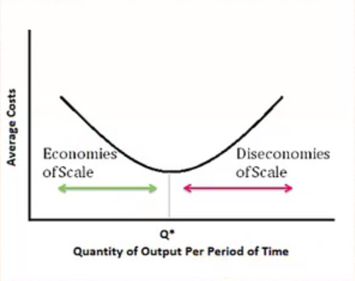
In the long run, we see that average costs, up to a certain point, fall as the business gets bigger and produces more. When this happens, they are said to experience economies of scale.
Once those average costs start rising, they experience diseconomies of scale. This occurs when they are not lowering their costs anymore from increasing the scale of production.
Therefore, the long run average cost curve will be u-shaped, as you can see below.

Up to point Q*, the firm experiences economies of scale because average costs are falling as they are achieving benefits from increasing scale of production. This is defined as an increase of operational facilities that create a decrease in marginal cost (or sometimes you will see this as average cost).
Beyond that point, the firm experiences diseconomies of scale or increasing cost, because of diminishing benefits from increasing scale of production. This is an increase of operational facilities that create an increase in marginal cost.
On the graph, for a very short amount of time, where the long run average cost curve may be flat--right around point Q*--would represent constant returns to scale. There is no change in average costs in this small region from increasing their scale of production.
So the economies of scale, as one of your key terms, is defined as an increase of operational facilities that create a decrease in marginal cost. Sometimes you'll see this as average cost. Whereas diseconomies of scale is an increase of operational facilities that create an increase in marginal or average costs.
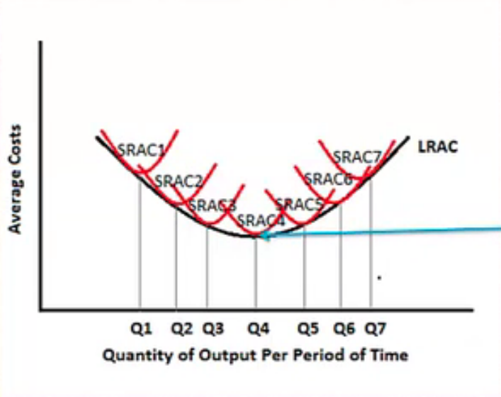
The long run average cost curve (LRAC) is made up of each of these short run average cost (SRAC) curves.

Ultimately, the goal is to find which of these scenarios--which scale of operation--will minimize average costs in the long run.
In the long run, the firm can adjust to changing market conditions and can make the best decision.
In this particular case, the best choice would be SRAC4.
Going back to our economies and diseconomies, the firm would experience economies of scale up to this point and diseconomies of scale beyond this point.
Now, how is it that the long run average cost curve is related to market structure?
Well, every firm does not have the same shape long run average cost curve.
It really varies among industries; even in the same industry, it will vary between companies.
It all has to do with differences in costs of production.
First of all, we know that we have fixed costs, and fixed costs are necessary for the production process to begin.
Now, sometimes these are sunk costs or upfront costs--sometimes called overhead--but they are not related to production levels.
They stay the same no matter how much the company produces. Therefore, the higher the production level, the more the company is able to spread out these fixed costs and achieve a lower average fixed cost per unit.
In fact, it is the variable costs that are related to production levels.
As the firm increases production, they will experience an increase in their variable costs. These will form the basis of defining whether the firm is seeing economies, constant, or diseconomies of scale.
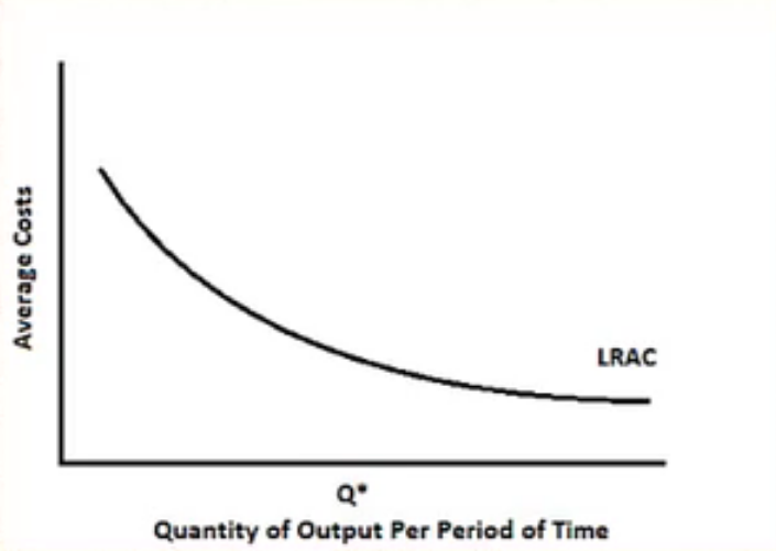
Here is an example of economies of scale as a barrier to entry.
Notice how this long run average cost curve is drawn so that it never experiences diseconomies of scale--average cost is constantly falling.

Utility companies provide a good example of economies of scale like this because they have enormous upfront fixed costs.
Depending on the utility company, most of them have a significant network that they have to put in place.
However, once that network is in place, the additional cost of servicing another home is fairly low as long as the network is in that area, and because of this, as they service more and more homes, their average costs fall, because their variable cost is not significantly increasing and they are able to spread out those initial upfront fixed costs.
Therefore, it makes sense for companies with large upfront costs to produce a lot.
Once the company is established--going back to our utility company example--it becomes very difficult to enter the market and compete because of the cost advantage the existing firm has from the economies of scale.
Even if another firm would try to enter, the competition might drive the price too low for either of them to realize any kind of profit.
This is why many utility companies are referred to as natural monopolies, where it simply makes sense for them to be the only company offering a utility in that area.
Therefore, the size of the existing firm becomes a barrier to entry.
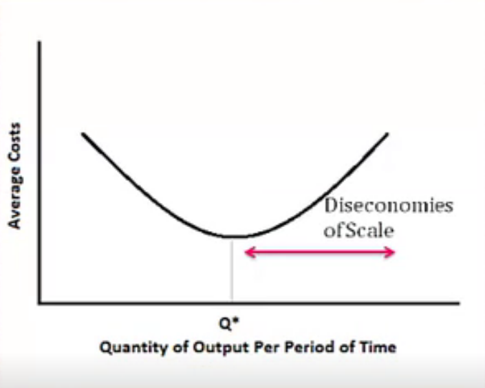
However, in more competitive industries, diseconomies of scale can occur.

It is possible for a firm to get too large, and certain inefficiencies can result, such as:
Therefore, it can become inefficient and average costs begin to rise.
In this graph, notice that the long run average cost curve is drawn such that the firm begins to experience diseconomies of scale at a fairly low level of output.
When this happens, it means there is an opportunity for new firms to enter easily--the opposite of what we covered in the section above.
Source: Adapted from Sophia instructor Kate Eskra.