Confidence Intervals

1. Confidence Intervals

Before we begin, it's important to note that sampling error is the inherent variability in the process of sampling. In a random sample, it occurs when you use a statistic, like a sample mean, to estimate the parameter, like a population mean. You won't always get exact accuracy with the sample mean, but you can use it to estimate the population mean. The idea is that you can be close.

When you take a larger sample, you're going to be, on average, closer. The sampling error, which is the amount by which the sample statistic is off from the population parameter, decreases. You get more consistently close values to the parameter when you take samples. When you calculate a margin of error in a study, you are approximating the sampling error.

When you take a sample, you try to obtain values that accurately represent what's going on in the population.

EXAMPLE

For example, suppose you took a simple random sample of 500 people getting ready for an upcoming election in a town of 10,000 and found that 285 of those 500 plan to vote for a particular candidate. Your best guess, for the true proportion, in the population of the town that will vote for candidate y is the proportion that you got in your sample—285 out of 500, which is 57% of the town. That's your best guess, but you might be off by a little bit.

You don't know if the true proportion of people who will vote for that candidate is 57%, and that's why you report a margin of error in your poll.

From the margin of error, you can create what is called a confidence interval. A confidence interval is an interval that contains the likely values for a parameter. We base the confidence interval on our point estimate, and the width of the interval is affected by the confidence level and sample size.

The confidence interval can be found using the following formula:

formula to know

Confidence Interval

The confidence interval is your point estimate, which is your best guess from your simple random sample, plus or minus the margin of error. You believe you are within a certain amount of the right answer with your point estimate.

term to know

Confidence Interval

An interval that contains likely values for a parameter. We base our confidence interval on our point estimate, and the width of the interval is affected by confidence level and sample size.

2. Margin of Error and the Effect of Confidence Level and Sample Size

The margin of error depends on two things:

• Sample size: You knew this from before when you said that a larger sample size results in less sampling error, and therefore, a lower margin of error.
• Confidence level: You're going to learn more about this, but a higher confidence level results in a larger margin of error.

EXAMPLE

If you want to be very confident that you're going to accurately describe what percent of people are going to vote for that particular candidate, you have to go out a little bit further on each side. Maybe you have to go out plus or minus 5%, as opposed to plus or minus 3%.

IN CONTEXT

95% Confidence

If the sampling distribution of p-hat is approximately normal, it will be centered at p, the population parameter; 95% of all sample proportions will be within two standard deviations of p.

So, p plus or minus two standard deviations will contain 95% of all p-hat. This is called 95% confidence. Approximately 19 out of every 20 samples, in the long term, that you take will be within two standard deviations of the right answer. Ninety-five percent of all p-hats are within two standard deviations of p.

If you want to be more confident, you can go out even further.

99% Confidence



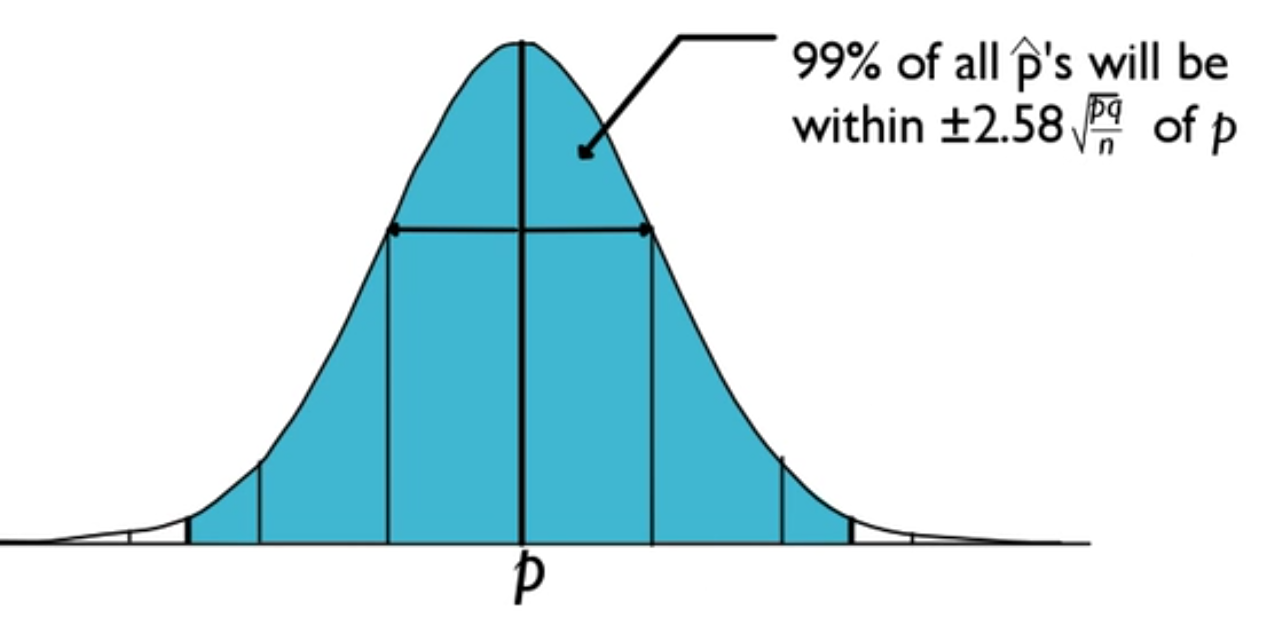
For instance, 99% of all p-hats will be within 2.58 standard deviations of p. This means that when you take a sample proportion, 99% of sample proportions will be within 2.58 standard deviations of the right answer, the value of p.

Take your p-hat value, and plus or minus 2.58 standard deviations, and you're 99% likely to capture the value of p.

3. Confidence Interval Formulas

When stating the confidence interval, we will use the following phrase:

In C% of samples, the parameter will be within z* standard errors of the sample statistic.

3a. For Sample Means

What does this look like if you're using means? If you are using means, it looks like that mu (μ), the parameter, will be contained in the interval statistic, which is x-bar, plus or minus z*, times the standard error of the statistic. In other words,

For C% of the time, the parameter μ will be contained in the interval

formula to know

Confidence Interval of Means

3b. For Sample Proportions

If you're using proportions, that means that the sample proportion, p-hat, plus or minus z* times the standard error, will contain the value of the parameter, p, some percent of the time, such as 95% or 99% of the time.

For C% of the time, the parameter p will be contained in the interval .

formula to know

Confidence Interval of Proportions

4. Finding Z*

The confidence level determines the value of z*. Depending on what you choose for your confidence level, z* will be affected that way. To find the z* critical value, we can use a z-table. For a confidence interval, we can follow the same steps as a two-sided test.

EXAMPLE

If we have a 95% confidence interval, this is actually the same as a 5% significance level. However, this is split between two tails, the lower and upper part of the distribution. Each tail will have 2.5%, or 0.025.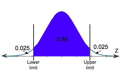

We can use the upper limit to find the critical z-score. Remember, a distribution is 100%, so to find the upper limit, we can subtract 0.025 from 1, which gives us 0.975. Now, we can use a z-table.

In a z-table, the value 0.975 corresponds with a 1.9 in the left column and 0.06 in the top row. This tells us that the z-score is 1.96.

Another way is to use a t-table, which you will learn more about in a later tutorial. We don't use the t-distribution for proportions; however, we can use the last row in this table to find the confidence levels.

Z confidence level critical values are found in the last row of this t-table, under the infinity value, or ">1000." Essentially, the normal distribution is the t-distribution with infinite degrees of freedom. We're going to look in this row to find the z-critical value that we should use, which is the same as the 1.96 we previously got.