Chi-Square Test for Goodness of Fit

1. The Chi-Square Distribution

Recall that the chi-square statistic is a particular test used to measure how the expected frequency differs from observed frequency.

Below is a visual representation of a chi-square distribution.

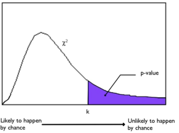
The chi-square distribution is a right-skewed distribution that generally measures the discrepancy from what a sample of categorical data would look like if you had an idea of what the population should look like in those categories.

• A smaller chi-square value would indicate a small discrepancy.
• A larger chi-square value would indicate a large discrepancy.

The p-value is always the area in the chi-square distribution to the right of your particular chi-square statistic that we end up calculating. The values on the left (low values of chi-square) are likely to happen by chance, and high values of chi-square are unlikely to happen by chance.

Just like the t-distribution, the chi-square distribution is actually a family of curves. The shape changes a little bit, based on the degrees of freedom, but it's always skewed to the right.

hint

The degrees of freedom for the chi-square distribution is the number of categories minus 1.

The conditions for using the chi-square distribution are:

• The data represent a simple random sample from the population.
• The observations should be sampled independently from the population, and the population is at least 10 times the sample size, which is called the "10% of the population" condition.
• The expected counts have to be at least 5. We have to ensure that the sample size is large, which is similar to the conditions for checking normality in other hypothesis tests.

---

2. The Chi-Square Test for Goodness of Fit

A chi-square test for goodness of fit is a method of testing the fit of three or more category proportions to a specified distribution. The null hypothesis is that the population distribution matches a specified distribution, while the alternative hypothesis is that the population does not match a specified distribution.

H₀: The population distribution matches a specified distribution.

H_a: The population distribution does not match a specified distribution.

As with any hypothesis test, you will need to follow these steps:

step by step

Step 1: State the null and alternative hypotheses.
Step 2: Check the conditions.
Step 3: Calculate the test statistic and p-value.
Step 4: Compare your test statistic to your chosen critical value, or your p-value to your chosen significance level. Based on how they compare, state a decision about the null hypothesis and conclusion in the context of the problem.

EXAMPLE

In the book Outliers, Malcolm Gladwell outlines a trend that he finds in professional hockey, related to birth month. Suppose a random sample of 512 professional hockey players was taken and their birth month was recorded.

Given the following information about birth month for the population, what would you expect for the number of hockey players born in each month?

Month	% of Population	Expected # of Hockey Players	Observed # of Hockey Players
January	8%		51
February	7%		46
March	8%		61
April	8%		49
May	8%		46
June	8%		49
July	9%		36
August	9%		41
September	9%		36
October	9%		34
November	8%		33
December	9%		30
Total			512

Are the recorded values what you would have expected, given the general population? It certainly appears that the earlier months of the year have larger numbers of NHL players born in them, which is not very consistent with the nearly uniform distribution of the population. The observed distribution looks like this:

What you would have expected is that of those 512 professional hockey players, 8% of them would have been born in January, 7% of them would have been born in February, etc. We can find the expected value for each month based on the given percentages of the population to get the following values:

Month	% of Population	Expected # of Hockey Players	Observed # of Hockey Players
January	8%	40.96	51
February	7%	35.84	46
March	8%	40.96	61
April	8%	40.96	49
May	8%	40.96	46
June	8%	40.96	49
July	9%	46.08	36
August	9%	46.08	41
September	9%	46.08	36
October	9%	46.08	34
November	8%	40.96	33
December	9%	46.08	30
Total		512	512

We would have expected 9% of the players to have been born in each of July, August, September, October, and December. So, we would have expected 46.08. However, apparently just 30 were born in December.

Let's perform a chi-square test for goodness of fit for this set of data to determine the discrepancy:

Step 1: State the null and alternative hypotheses.

• The null hypothesis, H₀, is that the distribution of birth month for the population of all hockey players is the same as the distribution for the entire population.
• The alternative hypothesis, H_a, is that the distribution of birth months for hockey players differs from that of the population.
• Significance level, α, can be set at 0.05, meaning if you get a p-value below 0.05, you'll reject the null hypothesis.

Step 2: Check the conditions.

Condition	Description
Simple Random Sample	You can treat it as such. This was a sample of hockey players born between 1980 and 1990. There's no reason to imagine that it's going to be particularly different or unrepresentative. Therefore, you can treat this as a random sample of players who have played or will play professional hockey.
Independence	You have to assume that there are at least 10 times as many players who have ever played pro hockey as there were in our sample, such that we can assume that independence piece. That would mean that you have to assume that there are at least 5,120 players who have ever played pro hockey.
Expected Counts At Least 5	The smallest number occurred in February, with 35.84. So, yes, when you look at the entire row of expected values, all of them are over 5.

Step 3: Calculate the test statistic and p-value.

Calculate your chi-square statistic using this formula:

formula to know

Chi-Square Test

The chi-square statistic is going to be the observed minus the expected for each month squared, divided by the expected for each month.

Month	Expected # of Hockey Players	Observed # of Hockey Players
January	40.96	51	2.46
February	35.84	46	2.88
March	40.96	61	9.80
April	40.96	49	1.58
May	40.96	46	0.62
June	40.96	49	1.58
July	46.08	36	2.20
August	46.08	41	0.56
September	46.08	36	2.20
October	46.08	34	3.17
November	40.96	33	1.55
December	46.08	30	5.61
Sum			34.21

When you add all of those components together, you get the chi-square value of 34.21.

In this case, it's also a good idea to state the degrees of freedom, which is the number of categories minus 1. There were 512 hockey players, but there were 12 categories. So, the degrees of freedom is 12 minus 1, or 11.

The p-value can be obtained from technology or with a table. When using a table, you go down to the line that corresponds with the degrees of freedom and look for the chi-square value.

χ2 Critical Values
Degrees of freedom (df)	Tail Probability Values, p
	0.250	0.200	0.150	0.100	0.050	0.025	0.020	0.010	0.005	0.0025	0.001	0.0005
1	1.32	1.64	2.07	2.71	3.84	5.02	5.41	6.63	7.88	9.14	10.83	12.12
2	2.77	3.22	3.79	4.61	5.99	7.38	7.82	9.21	10.60	11.98	13.82	15.20
3	4.11	4.64	5.32	6.25	7.81	9.35	9.84	11.34	12.84	14. 32	16.27	17.73
4	5.39	5.59	6.74	7.78	9.49	11.14	11.67	13.23	14.86	16.42	18.47	20.00
5	6.63	7.29	8.12	9.24	11.07	12.83	13.33	15.09	16.75	18.39	20.51	22.11
6	7.84	8.56	9.45	10.64	12.53	14.45	15.03	16.81	18.55	20.25	22.46	24.10
7	9.04	9.80	10.75	12.02	14.07	16.01	16.62	18.48	20.28	22.04	24.32	26.02
8	10.22	11.03	12.03	13.36	15.51	17.53	18.17	20.09	21.95	23.77	26.12	27.87
9	11.39	12.24	13.29	14.68	16.92	19.02	19.63	21.67	23.59	25.46	27.88	29.67
10	12.55	13.44	14.53	15.99	18.31	20.48	21.16	23.21	25.19	27.11	29.59	31.42
11	13.70	14.63	15.77	17.29	19.68	21.92	22.62	24.72	26.76	28.73	31.26	33.14
12	14.85	15.81	16.99	18.55	21.03	23.34	24.05	26.22	28.30	30.32	32.91	34.82
13	15.93	16.99	18.90	19.81	22.36	24.74	25.47	27.69	29.82	31.88	34.53	36.48
14	17.12	18.15	19.40	21.06	23.68	26.12	26.87	29.14	31.32	33.43	36.12	38.11

Going down to the line for 11 degrees of freedom, the closest to 34.21 is 33.14. This chi-square statistic corresponds with a probability of 0.0005. That's a very low p-value, much less than the significance level of 0.05.

Step 4: Compare your test statistic to your chosen critical value, or your p-value to your chosen significance level. Based on how they compare, state a decision about the null hypothesis and conclusion in the context of the problem.

Since your p-value of 0.0005 is low, you can't attribute the difference from the "norm" to chance alone.

This means that you must reject the null hypothesis in favor of the alternative and conclude that the distribution of birth months for professional hockey players differs significantly from the birth month distribution for the general populace.

IN CONTEXT

A manufacturing company claims that they expect five defects per day. This means that they believe the defects are evenly distributed across Monday through Friday.

A manager collects data on the days of the week and records the following information:

Day of the Week	Expected # of Defects	Observed # of Defects
Monday	5	6
Tuesday	5	8
Wednesday	5	4
Thursday	5	2
Friday	5	5

Let's perform a chi-square test for goodness of fit to determine if the variation that we see in the observation is from random chance, or if there is something different than an even distribution.

Step 1: State the null and alternative hypotheses.

We can state these hypotheses with a significance level of 5%:

Step 2: Check conditions. Let's check the three conditions for this hypothesis test.

• Simple Random Sample: We can assume that the manager collected data randomly throughout the days of the week.
• Independence: You have to assume that there have been at least 10 times as many defects at this manufacturing company as there were in our sample, such that we can assume that independence piece. That would mean that you have to assume that there have been at least 250 defects in this company's history.
• Expected Counts At Least 5: When you look at the entire row of expected values, all of them are 5, so this condition is satisfied.

Step 3: Calculate the test statistic and p-value.

We can use the chi-square formula to calculate the chi-square test statistic and take the observed minus the expected, then square those value and divide by the expected, and finally sum everything that we find.

Day of the Week	Expected # of Defects	Observed # of Defects
Monday	5	6
Tuesday	5	8
Wednesday	5	4
Thursday	5	2
Friday	5	5
Sum			4

The chi-square test statistic for this data set is equal to 4. We can use a chi-square table or technology to find the p-value that relates to this value of the chi-statistic, 4. We also need to look at the degrees of freedom, which is the sample size minus 1, or 5 minus 1. So, in this case, the chi-square statistic and the degrees of freedom are both 4. Applying this information and using technology, we find a p-value of 0.40601.

Step 4: Compare your test statistic to your chosen critical value, or your p-value to your chosen significance level. Based on how they compare, state a decision about the null hypothesis and conclusion in the context of the problem.

Remember, our significance level was 0.05. In this case, our p-value is greater than our significance level, so we cannot reject our null hypothesis.

term to know

Chi-Square Test for Goodness of Fit

A hypothesis test where we test whether or not our sample distribution of frequencies across categories fits with hypothesized probabilities for each category.