Calculating a T-Test Statistic

1. Conducting a T-Test

We're going to conduct a t-test for population means much like we conducted a z-test for population means. Recall that when running a hypothesis test, there are four parts:

step by step

1. State the null and alternative hypotheses.
2. Check the conditions necessary for inference.
3. Calculate the test statistic and its p-value.
4. Compare your test statistic to your chosen critical value, or your p-value to the significance level, and then based on how those compare, make a decision about the null hypothesis and a conclusion in the context of the problem.

The only difference between these two tests is the test statistic is going to be a t-statistic instead of a z-statistic. Because we’re using the t-distribution instead of the z- distribution, we're going to obtain a different p-value.

formula to know

T-Statistic for Population Means

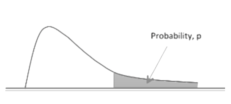
Therefore, we will need a new table—not the standard normal table for that. Below is the t-distribution table. We can see the possible p-values in the top row, and the t-values are the values inside the table. Potential p-values are based on the values within this section.

This distribution is actually one-sided, and it's the upper side that gives us these tail probabilities here. The entries in the t-table represent the probability of a value being above t.

The one new wrinkle that we're adding for a t-distribution is this value df (the far-left column). It's called the degrees of freedom. For our purposes, it's going to be the sample size minus 1. We find our t-statistic in whatever row our degrees of freedom is in. If it's between two values, that means our p-value is between these two p-values.

EXAMPLE

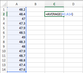
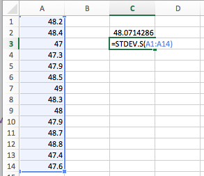
According to their bags, a standard bag of M&M's candies is supposed to weigh 47.9 grams. Suppose we randomly select 14 bags and got the following distribution.

48.2	48.4	47.0	47.3	47.9	48.5	49.0
48.3	48.0	47.9	48.7	48.8	47.4	47.6

Assuming the distribution of bag weights is approximately normal, is this evidence that the bags do not contain the amount of candy that they say that they do?

Step 1: State the null and alternative hypotheses.

The null is that the mean is 47.9 grams. The alternative is the mean is not 47.9 grams. We can select a significance level of 0.05, which means that if the p-value is less than 0.05, reject the null hypothesis.

• H₀: μ = 47.9; The mean of all M&M's bags is 47.9 g.
• H_a: μ ≠ 47.9; The mean of all M&M's bags is not 47.9 g.
• α = 0.05

Step 2: Check the necessary conditions.

Consider the following criteria for a hypothesis test:

Criteria	Description
Randomness	How was the data collected? The randomness should be stated somewhere in the problem. Think about the way the data was collected.
Independence	Population ≥ 10n You want to make sure that the population is at least 10 times as large as the sample size.
Normality	n ≥ 30 or normal parent distribution There are two ways to verify normality. Either the parent distribution has to be normal or the central limit theorem is going to have to apply. The central limit theorem says that for most distributions, when the sample size is greater than 30, the sampling distribution will be approximately normal.

Let's verify each of those in the M&M's problem:

• Randomness: It says in the problem that the bags were randomly selected.
• Independence: We're going to go ahead and assume that there are at least 140 bags of M&M's. That's 10 times as large as the 14 bags in our sample.
• Normality: Finally, it does say in the problem that the distribution of bag weights is approximately normal, so normality will be verified for our sampling distribution.

Step 3: Calculate the test statistic and the p-value.

Since we do not know the population standard deviation, we will calculate a t-test. We first need to find the sample mean and standard deviation. We can easily find both values by using Excel. First, list all the values given. To find the average, type "=AVERAGE(" and highlight all 14 values. We can also find this function under the Formulas tab and select the Math and Trigonometry option.



When we press "Enter," we get an average of 48.07. We can also find the standard deviation easily by typing "=STDEV.S(" and highlighting the 14 values. We can also find this function by going under the Formulas tab and then selecting the Statistical option.



This gives a standard deviation of 0.60.

Now, we can plug the known values into the t-statistic formula:


By plugging in all the numbers that we have, we obtain a t-statistic of positive 1.06. What exactly does this tell us? We need to calculate the probability that we get a t-statistic of 1.06 or larger.

In the table, we also need to identify the degrees of freedom (df), which is the sample size minus 1. The sample was 14 bags, so our degrees of freedom is 14 minus 1, or 13.

Let's look at the t-table in row 13 to find the closest value to 1.06:

T-Distribution Critical Values
Tail Probability, p
One-tail	0.25	0.20	0.15	0.10	0.05	0.025	0.02	0.01	0.005	0.0025	0.001	0.0005
Two-tail	0.50	0.40	0.30	0.20	0.10	0.05	0.04	0.02	0.01	0.005	0.002	0.001
df
1	1.000	1.376	1.963	3.078	6.314	12.71	15.89	31.82	63.66	127.3	318.3	636.6
2	0.816	1.080	1.386	1.886	2.920	4.303	4.849	6.965	9.925	14.09	22.33	31.60
3	0.765	0.978	1.250	1.638	2.353	3.182	3.482	4.541	5.841	7.453	10.21	12.92
4	0.741	0.941	1.190	1.533	2.132	2.776	2.999	3.747	4.604	5.598	7.173	8.610
5	0.727	0.920	1.156	1.476	2.015	2.571	2.757	3.365	4.032	4.773	5.893	6.869
6	0.718	0.906	1.134	1.440	1.943	2.447	2.612	3.143	3.707	4.317	5.208	5.959
7	0.711	0.896	1.119	1.415	1.895	2.365	2.517	2.998	3.499	4.029	4.785	5.408
8	0.706	0.889	1.108	1.397	1.860	2.306	2.449	2.896	3.355	3.833	4.501	5.041
9	0.703	0.883	1.100	1.383	1.833	2.262	2.398	2.821	3.250	3.690	4.297	4.781
10	0.700	0.879	1.093	1.372	1.812	2.228	2.359	2.764	3.169	3.581	4.144	4.587
11	0.697	0.876	1.088	1.363	1.796	2.201	2.328	2.718	3.106	3.497	4.025	4.437
12	0.695	0.873	1.083	1.356	1.782	2.179	2.303	2.681	3.055	3.428	3.930	4.318
13	0.694	0.870	1.079	1.350	1.771	2.160	2.282	2.650	3.012	3.372	3.852	4.221
14	0.692	0.868	1.076	1.345	1.761	2.145	2.264	2.624	2.977	3.326	3.787	4.140
15	0.691	0.866	1.074	1.341	1.753	2.131	2.249	2.602	2.947	3.286	3.733	4.073

In all likelihood, it's not one of the values listed in the row here, but rather between two values. We’ll see 1.06 is between the 0.870 and the 1.079, which means that the p-value is going to be between the two numbers 0.40 and 0.30 on the top row for a two-tailed test. Recall that we are testing to see if the mean weight of the M&M's bags is anything other than the hypothesized 47.9 grams, so this is a two-tailed test.

hint

You will need to consider if the problem is looking at a one-tailed or two-tailed test. If we need a value that is either less than or greater than the hypothesized mean, we will use a one-tailed test. If we are looking for any value that is different than the hypothesized mean, then we will use a two-tailed test.

Now, we can, in fact, use technology to nail down the p-value more exactly. We don't have to use this table, although we can still use the table to answer the question about the null hypothesis.

Step 4: Compare our p-value to our significance level.

We don't know exactly what our p-value is, but we know that it's within the range of 0.30 to 0.40. Since both of those numbers is greater than the significance level of 0.05, we're going to fail to reject the null hypothesis. There's our decision based on how they compare.

Finally, the conclusion is that there's not sufficient evidence to conclude that M&M's bags are being filled to a mean other than 47.9 grams.

try it

Emily is studying the effects of caffeine on cognitive performance. She’s particularly interested in whether coffee consumption impacts alertness levels among college students. To investigate, she conducts a study with a random sample of 50 students.
Sample Mean: The average number of cups of coffee consumed per day by her sample is 3.8 cups.
Sample Standard Deviation: 1.2 cups

Emily wants to compare her sample to the general population’s average coffee consumption, which is 3.0 cups per day.

Calculate Emily's t-statistic.

Apply the formula for the t-statistic of sample means:

Interpret Emily's t-statistic.

Use the t-table for 49 degrees of freedom (50 is close enough) and find the p-value for the two-tailed distribution because she wants to know the likelihood her sample consumption is different (higher or lower) than the population. In this case, our p-value is <0.001, which means Emily can reject her null hypothesis.

term to know

T-Test for Population Means

The type of hypothesis test used to test an assumed population mean when the population standard deviation is unknown. Due to the increased variability in using the sample standard deviation instead of the population standard deviation, the t-distribution is used in place of the z-distribution.