Table of Contents |
Suppose we want to calculate the area between the graph of a nonnegative function  and the x-axis interval
  as shown in the figure below.
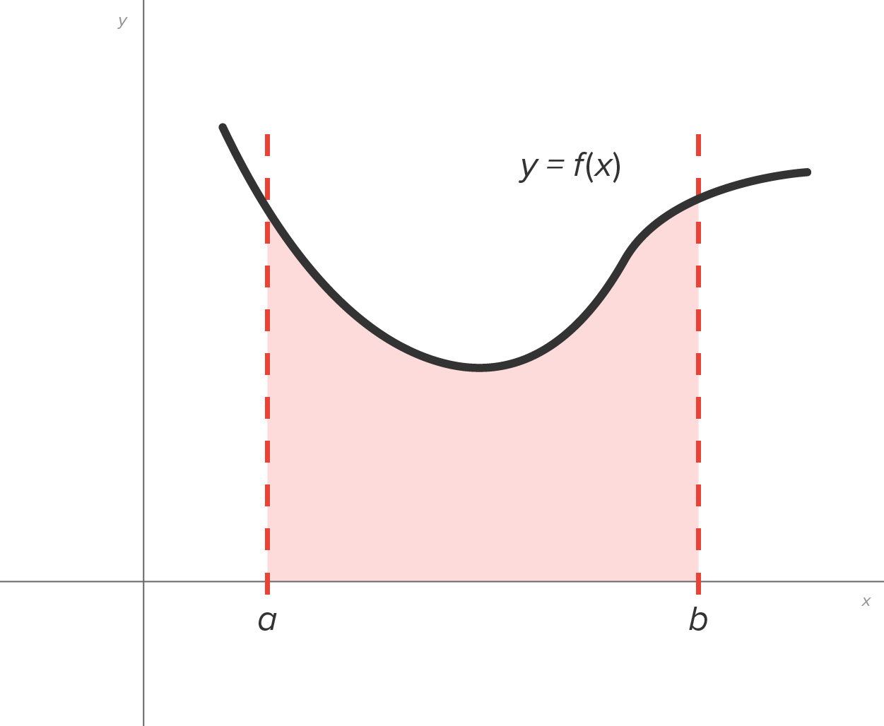
If is nonnegative, the Riemann sum method is to build several rectangles with bases on the interval  and sides that reach up to the graph of
  Then, the areas of the rectangles can be calculated and added together to get a number called a Riemann sum of on

The area of the region formed by the rectangles is an approximation of the area between the graph and the x-axis.
In order to find the Riemann sum, there are several quantities that need to be established first.
First, a partition of the interval is needed to establish the bases of the rectangles. Consider the graph in the figure.

The endpoints of the interval are  and
and  . In order to form three rectangles, two more values
( and
and  ) are added to form a partition of the interval
We label the partition by the x-coordinates, namely  The numbers are listed in increasing order.
Note that there are 4 x-values in the partition for three rectangles. In general, if n rectangles are desired, there would be n + 1 x-values in the partition. This is why the first one is labeled as (which is the left-hand endpoint of the interval), so the last one can be called  (to match the number of rectangles).
The subintervals for this partition are 
 and
and 
into smaller intervals. It is most convenient to select a partition where each x-value is the same distance apart from its neighbor, but that is not necessary.
Continuing with this partition, we use the notation  to represent the width of the
  subinterval. Recall that the width of an interval is the difference between its endpoints.
| Subinterval | Width |
|---|---|

|

|

|

|

|

|
Let  the value of x used in the subinterval. There are popular choices for
Consider the figure shown below:
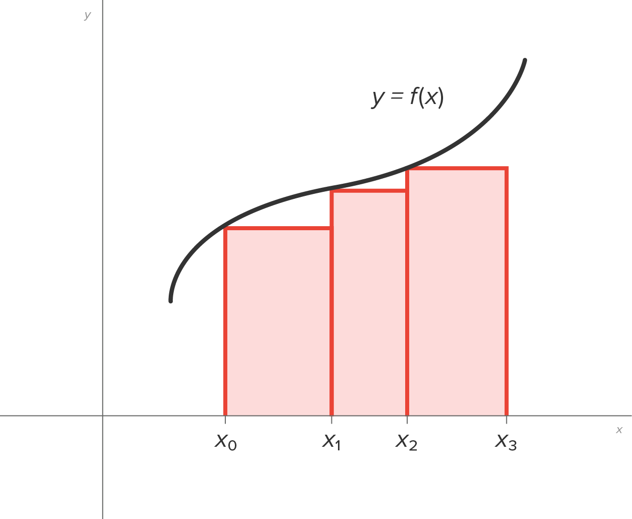
As the rectangles suggest, the left-hand endpoint was used in each sub-interval to set the height of the rectangle. This means:
| Subinterval | Value Chosen | Width |
|---|---|---|
|
|

|
|
|
|

|
|
|
|

|
|
So, we can say:


 and the x-axis is the sum of these areas. Written using sigma notation, the Riemann sum is:

In general, here is the definition (formula) for a Riemann sum.
 and the x-axis by using n rectangles, the summation
  is called the Riemann sum, where
  is a value of x in the subinterval, and is the width of the subinterval.
Now that we have all the definitions, let’s compute a few Riemann sums.
EXAMPLE
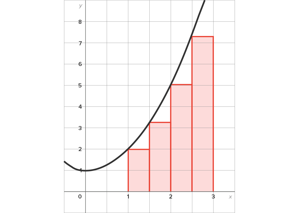
Use a Riemann sum with 4 rectangles of equal width to approximate the area between and the x-axis on the interval
  Use the left-hand endpoint of each subinterval.

| Subinterval | Width of Subinterval | Value Chosen in Each Subinterval |
|---|---|---|

|
0.5 | 1 |

|
0.5 | 1.5 |

|
0.5 | 2 |

|
0.5 | 2.5 |

|
Use the Riemann sum formula. |

|
Factor out 0.5. |

|
Substitute values:    
|

|
Simplify. |

 since they are all the same, then
  and the x-axis on the interval Use the right-hand endpoint of each subinterval. Note, this is the same information as in the last example, except that right-hand endpoints are used.
 we have
  and
and 

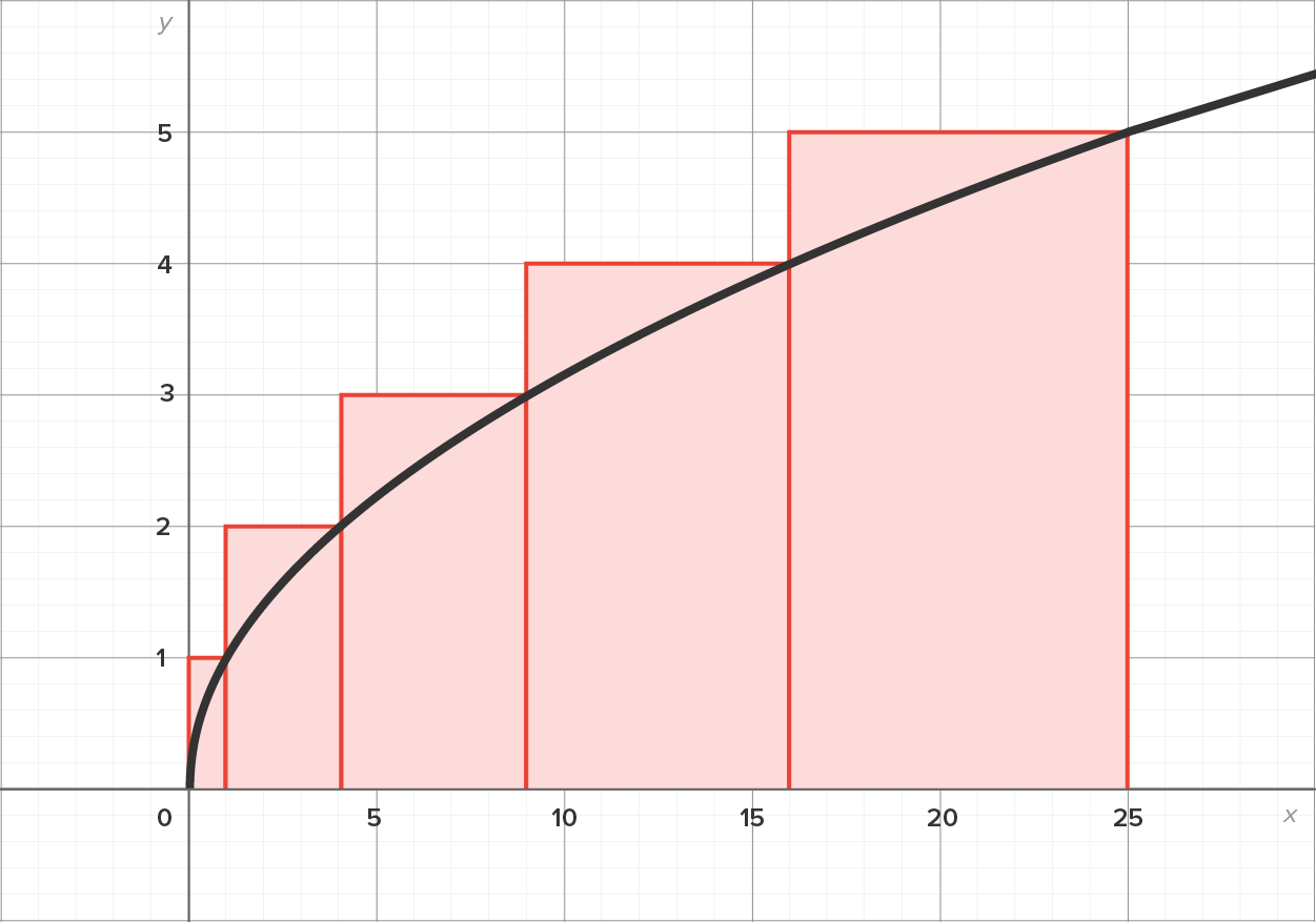
Let’s look at an example where the widths of the intervals are not the same.
EXAMPLE
Consider the function on the interval
  Estimate the area between and the x-axis by using the partition
  Use the right-hand endpoint of each subinterval.
| Subinterval | Width of Subinterval | Value Chosen in Each Subinterval |
|---|---|---|

|
1 | 1 |

|
3 | 4 |

|
5 | 9 |

|
7 | 16 |

|
9 | 25 |
along with the rectangles is shown below.


|
Use the Riemann sum formula. |

|
Substitute values:     
|

|
Simplify. |

 on the interval
  using 4 rectangles of equal width, using the left-hand endpoints of each subinterval.
and the x-axis on the interval , by obtaining the sum from the areas of rectangles. You learned that when finding the Riemann sum, there are several quantities that need to be established first: find the partition and subintervals; find the width of each subinterval; select x-values within each partition; and finally, form the Riemann sum. Using this knowledge, you were then able to explore several examples of using Riemann sums to calculate area. Many applications we will investigate later in this course are based on Riemann sums, which makes this a very important topic to understand.
using 4 rectangles of equal width, using the left-hand endpoints of each subinterval.
and the x-axis on the interval , by obtaining the sum from the areas of rectangles. You learned that when finding the Riemann sum, there are several quantities that need to be established first: find the partition and subintervals; find the width of each subinterval; select x-values within each partition; and finally, form the Riemann sum. Using this knowledge, you were then able to explore several examples of using Riemann sums to calculate area. Many applications we will investigate later in this course are based on Riemann sums, which makes this a very important topic to understand.
Source: THIS TUTORIAL HAS BEEN ADAPTED FROM CHAPTER 4 OF "CONTEMPORARY CALCULUS" BY DALE HOFFMAN. ACCESS FOR FREE AT WWW.CONTEMPORARYCALCULUS.COM. LICENSE: CREATIVE COMMONS ATTRIBUTION 3.0 UNITED STATES.
A set of x-values that are used to split the interval  into smaller intervals.
The sum obtained from the areas of rectangles that are used to approximate the area between a curve and the x-axis.
A smaller interval that is part of a larger interval.
When approximating the area between a nonnegative function  and the x-axis by using n rectangles, the summation
  is called the Riemann Sum, where
  is a value of x in the
  subinterval, and
  is the width of the
  subinterval.
