Approximating Definite Integrals

1. Approximating a Definite Integral Using Rectangles

When you combine our knowledge of antiderivatives with the tables of integrals from the last tutorial, there are still functions for which we do not know antiderivatives.

EXAMPLE

cannot be evaluated exactly since the antiderivative of can’t be written in terms of the functions we are familiar with in calculus.

Recall in challenge 5.2, we approximated definite integrals by using rectangles of equal width along the x-axis.

Consider a nonnegative function on the interval Break the interval into n equal subintervals; then, each subinterval has width

Note, these approximation methods can be used whether is positive, negative, or both on the interval We are considering only nonnegative functions for now to make the visual connection with the area between and the x-axis on

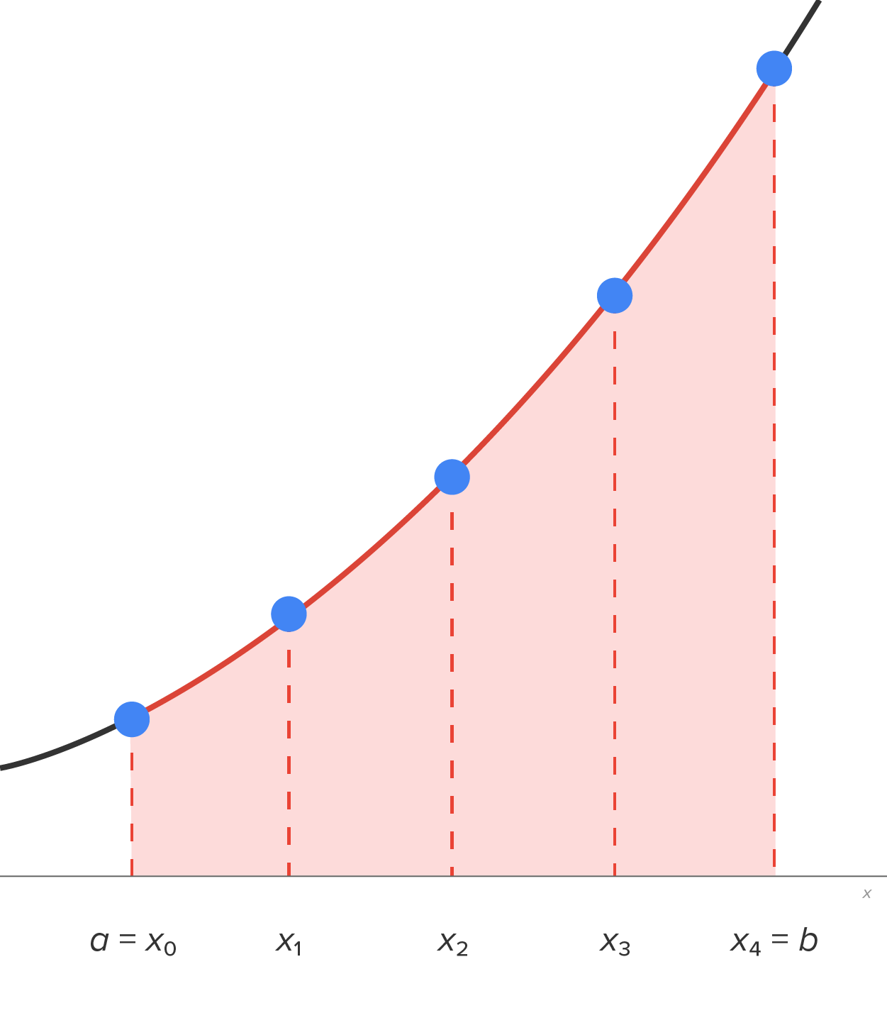
The graph below shows the interval broken into 4 subintervals, where the left-hand endpoints are used to determine the height of each rectangle.

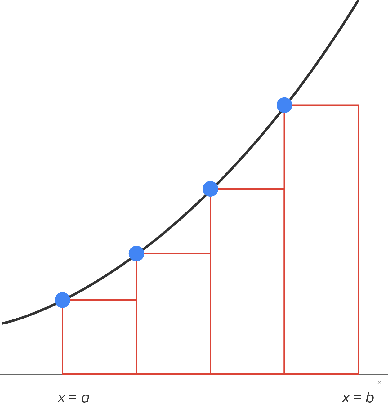
Naturally, as the number of rectangles (subintervals), n, gets larger, the approximation gets closer to the actual area (in this case, also the definite integral).

Now that we have our framework, let’s look at an example where we use all three approximation methods.

EXAMPLE

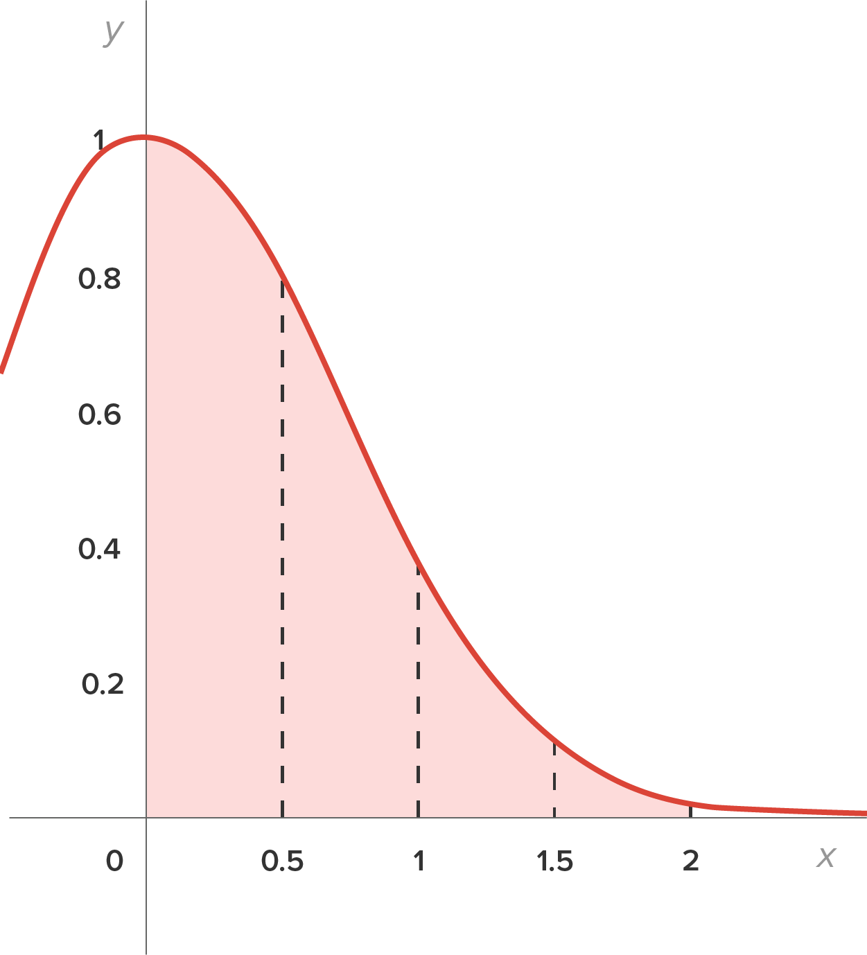
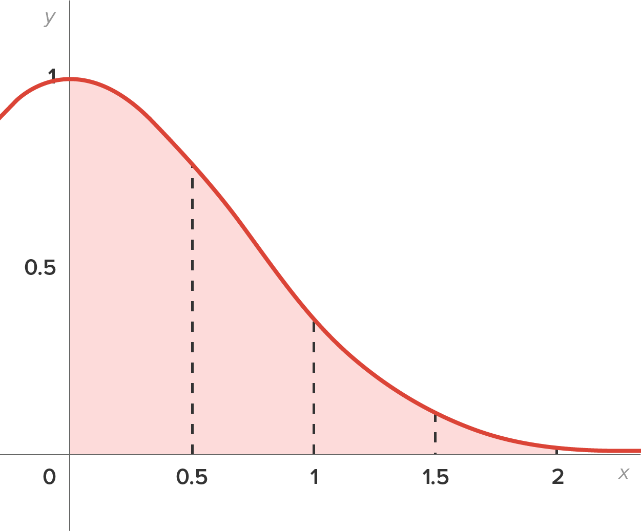
Estimate the value of by using subintervals of equal width using (a) left-hand endpoints, (b) right-hand endpoints, and (c) midpoints of each subinterval.

The graph of the region is shown in the figure below. Note: This means the subintervals are and

Points	Value
Left-hand endpoints	Using the left-hand endpoint of each interval, this means the x-values are 0, 0.5, 1, and 1.5. Then, the estimate for the definite integral is Note that we can factor out 0.5: After using a calculator, this is approximately 1.12604 (to five decimal places).
Right-hand endpoints	Using the right-hand endpoint of each interval, this means the x-values are 0.5, 1, 1.5, and 2. Then, the estimate for the definite integral is Note that we can factor out 0.5: After using a calculator, this is approximately 0.63520 (to five decimal places).
Midpoints	Using the midpoint of each interval, this means the x-values are 0.25, 0.75, 1.25, and 1.75. Then, the estimate for the definite integral is Note that we can factor out 0.5: After using a calculator, this is approximately 0.88279 (to five decimal places).

Looking at the region, the left-hand endpoints produce an overestimate and the right-hand endpoints produce an underestimate. It is more difficult to tell if the midpoint estimate is higher or lower than the actual value, but one thing is for sure: it is closer to the actual than the others.

For your reference, so the midpoint estimate was very close!

To account for the left-hand and right-hand endpoints providing overestimates or underestimates, sometimes the average of the left-hand and right-hand estimates is used.

In this case, this average is which is indeed closer.

try it

Consider

Using subintervals, estimate the definite integral using left-hand endpoints, right-hand endpoints, and midpoints of each subinterval. Round each estimate to 5 decimal places.

Estimate using left-hand endpoints.

Let

With subintervals,

Breaking the interval into 4 equal pieces, the endpoints are 1, 1.5, 2, 2.5, and 3.

The left-hand endpoints of each subinterval are

Then, the estimate of the definite integral using left-hand endpoints is:

Estimate using right-hand endpoints.

Let

With subintervals,

Breaking the interval into 4 equal pieces, the endpoints are 1, 1.5, 2, 2.5, and 3.

The right-hand endpoints of each subinterval are

Then, the estimate of the definite integral using right-hand endpoints is:

Estimate using midpoints.

Let

With subintervals,

Breaking the interval into 4 equal pieces, the endpoints are 1, 1.5, 2, 2.5, and 3.

The midpoints of each subinterval are

Then, the estimate of the definite integral using midpoints is:

2. Approximating a Definite Integral Using Trapezoids (Trapezoidal Rule)

Consider the region shown in the figure, this time connecting consecutive points with a line.

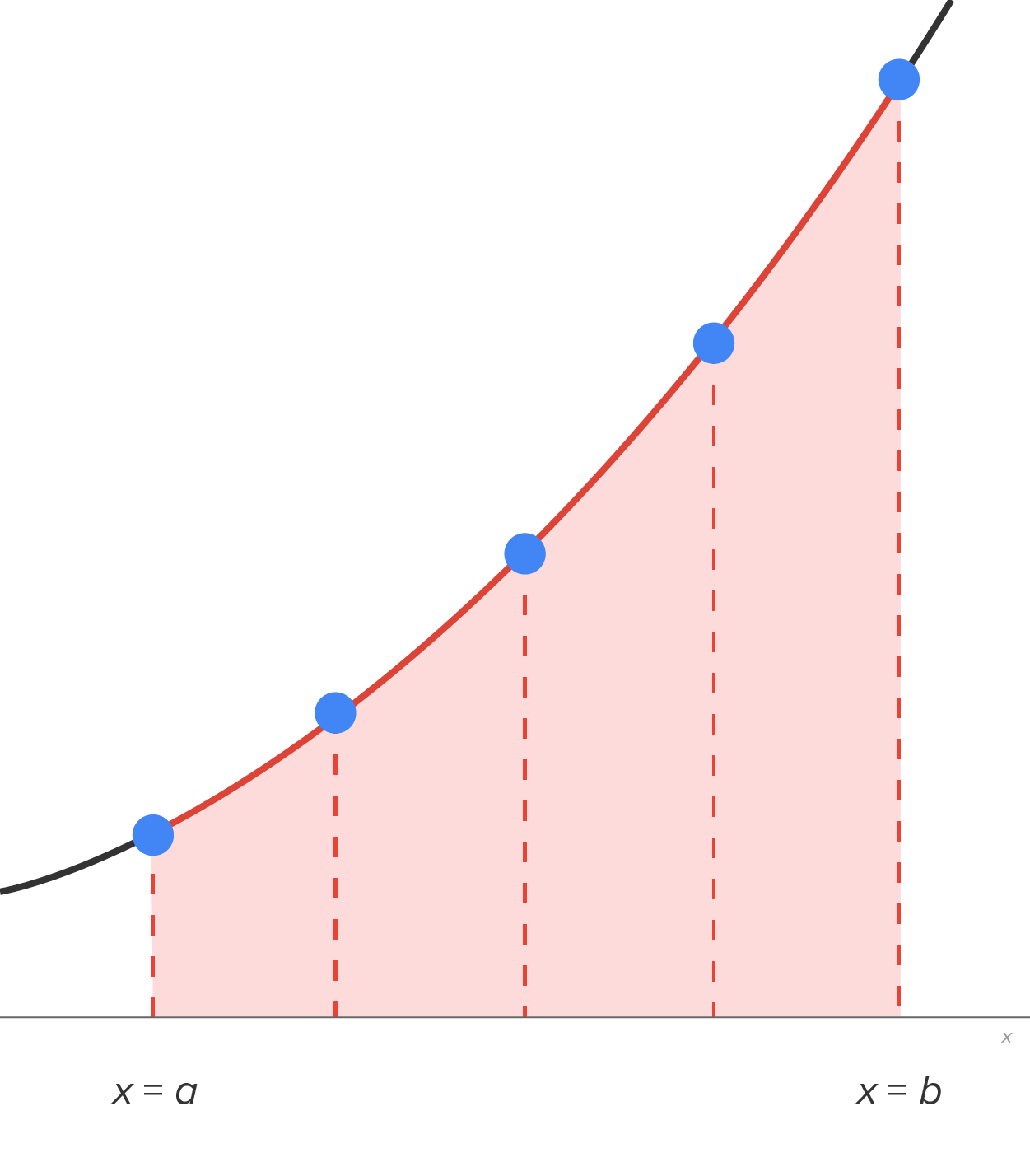
This means that trapezoids are used to approximate the area of the region in each subinterval. Recall that the area of a trapezoid is where h is the height (the distance between the parallel sides) and and are parallel bases.

In this case, the height is the width of each trapezoid and the bases are the function values on both sides.

Let the right-hand endpoint of each subinterval, and

Trapezoid	Bases	Height	Area
First trapezoid on the interval	and
Second trapezoid on the interval	and
Third trapezoid on the interval	and
Last trapezoid on the interval	and

Notice that the endpoints (a and b) are only used in one trapezoid each. All the interior values of x are used in two trapezoids.

To estimate (assuming is nonnegative), add all the areas together:

Notice that each quantity has a factor of We’ll factor this out:

There are some like terms within the brackets. Combine them:

Note: we know that the term will show up twice since it is a base in each of the last two trapezoids.

This leads to a formula for estimating using trapezoids. This method is aptly named the trapezoidal rule.

formula to know

Trapezoidal Rule

can be approximated by the sum where and are the endpoints of each equally spaced subinterval.

big idea

The estimate obtained from the trapezoidal rule is actually the average of the left- and right-hand endpoint rules. Thus, if you have the left- and right-hand estimates already calculated, the trapezoidal estimate follows quickly.

EXAMPLE

Estimate the value of by using subintervals of equal width using the trapezoidal rule. Check that this is equal to the average of the left- and right-hand endpoint estimates.

The graph of the region (with trapezoids drawn) is shown in the figure below. Note: This means the subintervals are and



The x-values used are x = 0, 0.5, 1, 1.5, and 2.

Then, the estimate for the definite integral is:




After using a calculator, this is approximately 0.88062 (to five decimal places).

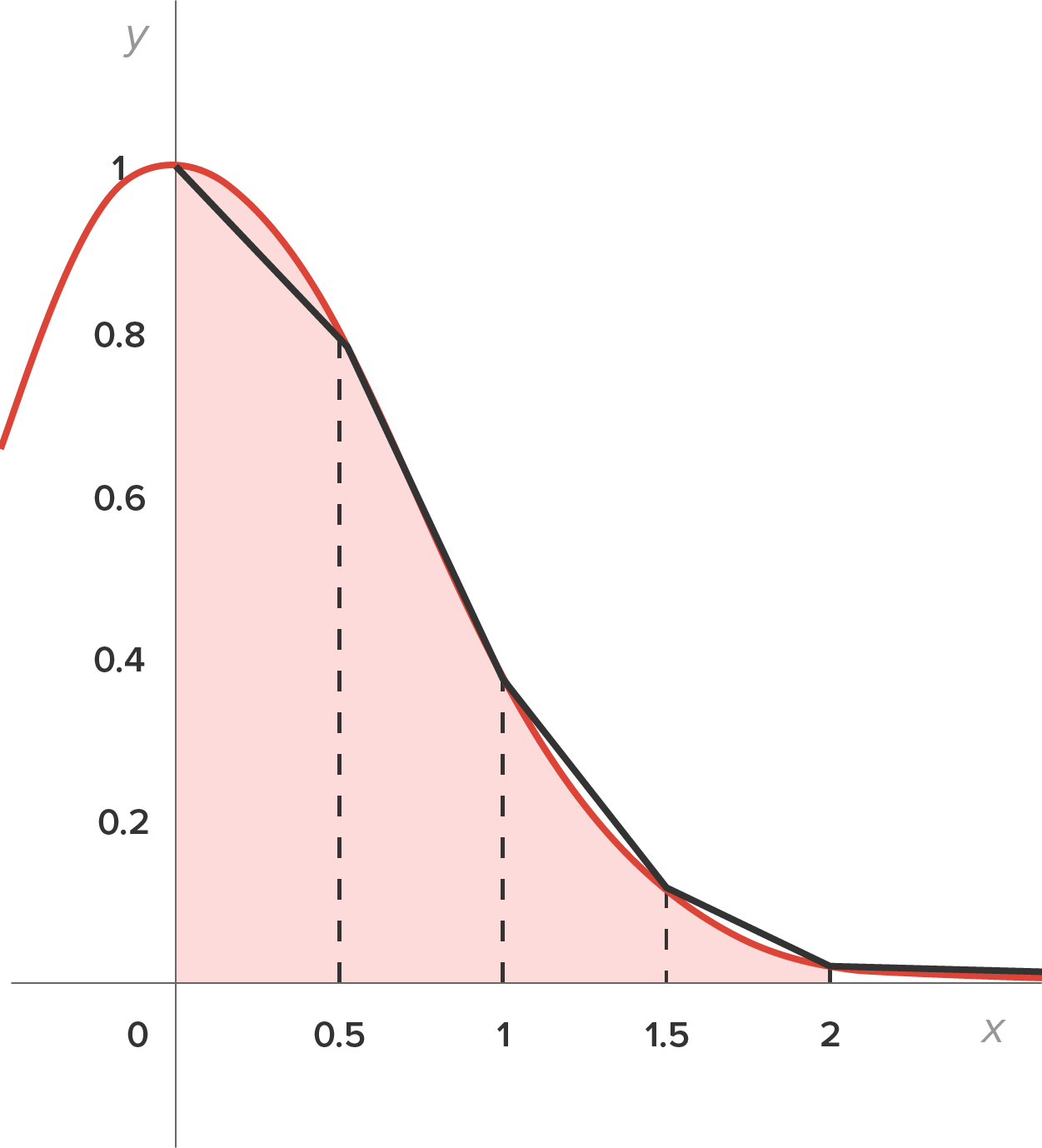
In an earlier example, we also computed the average of the left- and right-hand estimates, and this was also approximately 0.88062. (If you look beyond the third decimal place in each, the estimates should be identical.)

try it

Consider

Using n = 4 subintervals, estimate the definite integral using the trapezoidal rule. Round your answer to 5 decimal places.

Let

With subintervals,

Breaking the interval into 4 equal pieces, the endpoints are 1, 1.5, 2, 2.5, and 3.

By the trapezoidal rule, the integral estimate is:

3. Approximating a Definite Integral Using Parabolas (Simpson’s Rule)

While the methods discussed so far seem to do a fair job of approximating it makes more sense to approximate with a curve rather than a straight line (if is a straight-line function, there is no need to approximate the definite integral). To that end, we can also use parabolas, but not before we establish a rule for the definite integral of a parabola.

If then

Now, consider this region.

If we want to approximate by using a parabola, we would have

Note: (that is, since the x-values are evenly spaced, is the average of and ).

Also, consider the quantity Since is the distance between two consecutive x-values, it follows that which means

Thus, we can write

Then, considering the interval we have

Then, the approximation for is the sum of the previous two approximations:

That is,

Factoring out this becomes

Combining like terms, this becomes

Note: since each parabola uses two subintervals, the number of subintervals must be even.

If this process were to continue, notice the following:

• and would have coefficients of 1.
• ... would have coefficients of 4 (odd-numbered subscripts).
• ... would have coefficients of 2 (even-numbered subscripts, but not the endpoints).

This approximation method is known as Simpson’s rule.

formula to know

Simpson's Rule

The value of is approximated by where and are the endpoints of each equally spaced subinterval. Note: n must be even.

EXAMPLE

Estimate the value of by using subintervals of equal width using Simpson’s rule.

The graph of the region is shown in the figure. Note: . This means the subintervals are and



The x-values used are x = 0, 0.5, 1, 1.5, and 2.

Then, the estimate for the definite integral is:



After using a calculator, this is approximately 0.88181 (to five decimal places).

Comparing this to the left-hand, right-hand, midpoint, and trapezoidal estimates, these are all very close, but it turns out that Simpson’s rule gives the closest approximation for this function on this interval. In general, Simpson’s rule usually gives the best estimate out of the five we discussed, but there are exceptions.

try it

Consider

Using n = 4 subintervals, estimate the definite integral using Simpson’s rule.

Let

With subintervals,

Breaking the interval into 4 equal pieces, the endpoints are 1, 1.5, 2, 2.5, and 3.

By Simpson’s rule, the integral estimate is:

The approximation methods shown in this challenge are all used to approximate the value of a definite integral. Using that connection, these methods can be used to approximate the area of an irregularly shaped region, as we’ll see in the next part.

4. Application: Approximating Area

EXAMPLE

Suppose the measurements of a park are shown below. What is the approximate area of the park? As the figure suggests, the measurements were taken every 30 feet.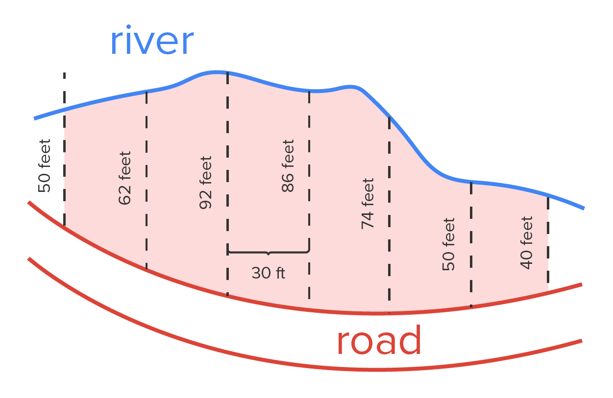



Let the length of the park at a distance of x feet from the left-hand side (as shown). Then, the area of the park is (there are 6 widths of 30 feet, for a total of 180 feet).

Since we don’t have an expression for we’ll need to use the approximation techniques learned in this section to estimate the area.

Using with subintervals, we can easily use the left-hand and right-hand endpoints, the trapezoidal rule and Simpson’s rule to approximate the area. (Since we don’t know the values of in the middle of each interval, the midpoint method cannot be used.)

Here is a table of values for all the values of x.

	0	30	60	90	120	150	180
Length	50	62	92	86	74	50	40

Below is a table that shows the various approximations for the area. Notice that the estimates are fairly close to each other.

Method	Estimation for the Area
Left-Hand Endpoints
Right-Hand Endpoints
Trapezoids
Simpson's Rule

try it

Consider the pond shown in the figure below. Assume each subinterval is 5 feet wide and that the distance across at the endpoints is 0 feet.

Use left- and right-hand endpoints, the trapezoidal rule, and Simpson’s rule to estimate the surface area of the pond.

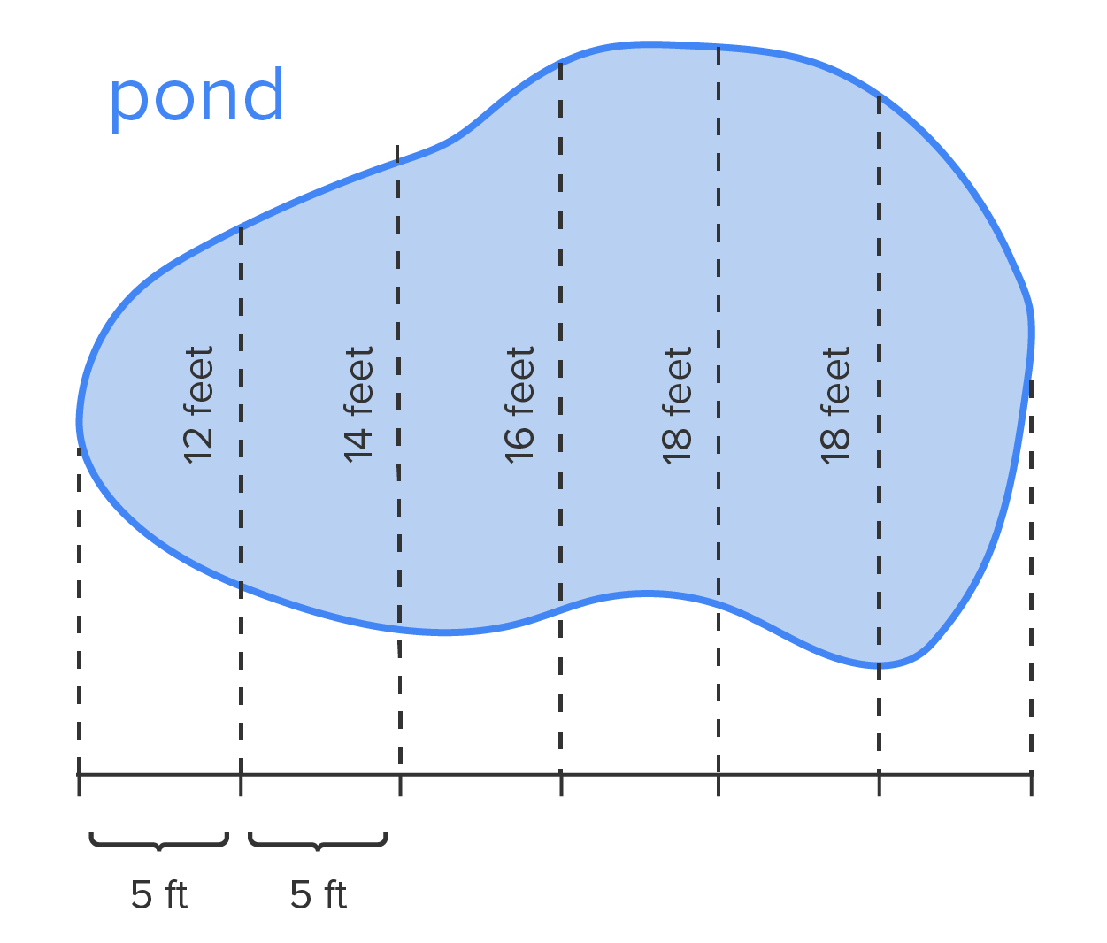Let the length of the lake at a distance of x feet from the left-hand side.

Then, gives the area of the lake.

To approximate this integral, we are using 6 equal subintervals of width 5. This means and

The lengths of the lake at each given point can be summarized by the table:

x	0	5	10	15	20	25	30
f  (x  )	0	12	14	16	18	18	0

Left-hand estimate:

Right-hand estimate:

Trapezoidal estimate:

Simpson’s Rule Estimate:

summary

In this lesson, you learned that when approximating definite integrals, there are several methods that can be used: using rectangles, using trapezoids (trapezoidal rule), and using parabolas (Simpson's rule). The key takeaway here is the progression. Using rectangles is simpler, but doesn’t give as good an estimate as trapezoids, which still has flaws since a line is used to approximate a curve. Simpson’s rule, using parabolas, seems to be the best match for a curve but since not all curves are parabolic, there is still room for some error. In all cases, the estimate is improved by increasing the number of subintervals. Finally, you were able to apply the techniques learned in this section to approximate the area in several examples.