In this lesson, you will learn how to test if differences exist among three or more population means by applying an ANOVA analysis. Specifically, this lesson will cover:
-
This lesson builds on key concepts from an Introduction to Statistics course. Specifically, this tutorial assumes familiarity with the foundational idea of ANOVA.
1. Introduction to ANOVA
Since you have just learned how to compare two means for two populations using the two-sample t-test, you are in a great spot to extend your knowledge to ANOVA (Analysis of Variance). ANOVA allows you to compare the means of three or more groups simultaneously, helping you determine if there are any statistically significant differences among them.
Imagine you work for a company called SalesPro Inc., and you want to find out if different sales teams have different average monthly sales. The company has three sales teams:
- Team Alpha
- Team Beta
- Team Gamma
You want to see if there is a significant difference in the average monthly sales among these three teams.
ANOVA will tell you if the differences in average sales are statistically significant. This means it will show if at least one team’s sales are different from the others in a meaningful way.
If ANOVA shows a significant difference, you can conclude that at least one sales team is performing differently. This insight helps SalesPro Inc. understand which teams might need more training or resources and which strategies are working best.
Now, since you just learned about two-sample t-tests, you might be thinking about comparing the sales of each team on a pairwise basis. For example, you could compare:
- Team Alpha vs. Team Beta
- Team Alpha vs. Team Gamma
- Team Beta vs. Team Gamma
While this approach can work, it has some limitations. Performing multiple t-tests increases the risk of
Type I errors (false positives), where you might incorrectly conclude that there is a significant difference when there is not one. This is where ANOVA comes in handy. ANOVA allows you to compare all three teams simultaneously, reducing the risk of errors and providing a more comprehensive analysis. In the next section, you will learn how ANOVA works.
-
- Type I Error
- An error that occurs when you incorrectly reject the null hypothesis, concluding that there is a significant difference between groups when, in reality, there is not one.
1a. Steps in ANOVA
Conducting an ANOVA analysis involves several key steps. Below is a guide to help you understand the process.
-
1.
State the Hypotheses: Clearly define the null and alternative hypotheses.
The hypotheses in ANOVA are:

The null hypothesis states all group means are equal. In other words, there is no significant difference among the means of any of the
k groups.
The alternative hypothesis states that at least one group mean is different from the others. This means that there is a significant difference among the means of the groups.
2.
Gather the Data: Gather data in a way that is designed to test the hypotheses.
3.
Choose the Significance Level: Decide on the α level (for example, 0.05 or 0.10).
4.
Perform a Statistical Test: You will use an F-test statistic to perform an ANOVA.
The F-test statistic is a value that will be computed when the ANOVA test is run. Imagine you have four different brands of cereal, and you want to know if people like one brand more than the others. You ask a bunch of people to rate each brand. The F-statistic helps you figure out if the differences in ratings are just by chance or if they are really different.
Below is how the F-test statistic works in the ANOVA test in the context of the cereal example.
Calculate the Variance: First, you look at how much the ratings vary within each brand (this is called “within-group variance”) and how much the ratings vary between the different brands (this is called “between-group variance”).
Compare the Variances: The F-statistic is the ratio of the between-group variance to the within-group variance. If the F-statistic is large, it means the differences between the groups are bigger than the differences within each group.

-
Large F-statistic: This suggests that the differences between the groups are significant, providing more support to reject the null hypothesis (which states that there are no differences between the groups).
-
Small F-statistic: This indicates that the differences between the groups are not significant, leading you to fail to reject the null hypothesis.
How ‘large’ does the F-statistic have to be for you to reject the null hypothesis? This is what the p-value tells you.
Check the Significance with the p-value:
-
Small p-value (usually ≤ 0.05): Indicates that the F-statistic is large enough to suggest that the differences among the groups are unlikely to be due to random chance. This means the differences are statistically significant.
-
Large p-value (usually > 0.05): Indicates that the F-statistic is not large enough to rule out random chance as the reason for the differences among the groups. This means the differences are not statistically significant.
Make a Decision:
-
Reject the null hypothesis: If the p-value ≤ α (level of significance), reject the null hypothesis.
-
Fail to reject the null hypothesis: If the p-value > α (level of significance), fail to reject the null hypothesis.
Interpret the Results: Explain the results of the hypothesis test in the context of the business problem.
For example, suppose the ANOVA test for the mean ratings among the four cereals found the F-statistic was large and the corresponding p-value was small (less than 0.05), you would reject the null hypothesis. This result means that there are significant differences in the ratings between the cereal brands.
The business conclusion would be that certain cereals are preferred over others. Some actionable insights that could be taken include:
- Focus marketing efforts on the preferred brands to capitalize on their popularity.
- Investigate what makes the preferred brands more appealing and apply those insights to improve or innovate other products.
- Adjust production and stocking levels to meet the demand for the more popular brand.
1b. ANOVA Example
Let’s look at how you would apply an ANOVA in a real-world business scenario.
-
EXAMPLE
A social media company wants to analyze the engagement of three different types of posts: Memes, Educational, and Promotional. They collected the number of likes each type of post has received over the past year.
Your job is to determine if there are significant differences in the average number of likes between the three types of social media posts: Memes, Educational, and Promotional.
In performing this ANOVA test, you will complete the following steps.
Step 1: State the Hypotheses
- H₀:
 (no difference in the average number of likes between the three types of posts)
- H₁: at least one
 is different (at least one type of post has a different average number of likes compared to the others)
Step 2: Gather the Data
The
social_media_engagement.xlsx Excel file contains engagement data for the three different types of social media posts: Memes, Educational, and Promotional. Each type of post has a sample of 50 rows, and each row is the number of likes for the corresponding type of post.
Step 3: Choose a Significance Level
Use a level of significance,
 Step 4: Perform a Statistical Test
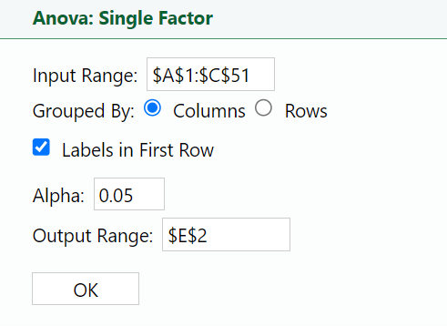
You will complete this step by running an ANOVA test in Excel. Perform the following:
1. Select
ANOVA: Single Factor. The dialog box opens.
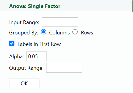
2. Place your cursor in the
Input Range: box and select the data in columns A-C.
3. Place your cursor in the
Output Range: box, select cell E2 in the Excel worksheet, and select
OK.
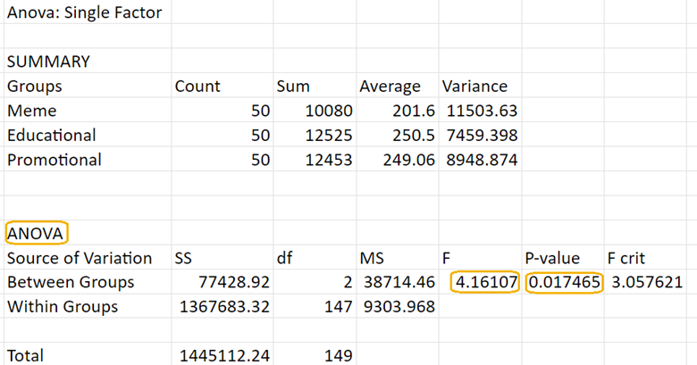
You will obtain the following output in Excel. The output contains two parts: SUMMARY and ANOVA. The SUMMARY portion provides a snapshot of the basic descriptive statistics for each group. The ANOVA portion contains the results of the ANOVA test, which helps you determine if there are significant differences between the groups.
Let's focus on the ANOVA portion.
Below is a short description of each part of the ANOVA table.
1.
Source of Variation:
-
Between Groups: This shows the variation due to differences between the group means (that is, differences in likes between Memes, Educational, and Promotional posts).
-
Within Groups: This shows the variation within each group (that is, how much likes vary within Memes, within Educational posts, and within Promotional posts).
2.
Sum of Squares (SS):
-
Between Groups SS: Measures the variability due to the differences between the group means. In this context, it represents how much the average number of likes differs between the three types of posts (Memes, Educational, and Promotional).
-
Context: Imagine you have the average number of likes for each type of post. The Between Groups SS tells us how much these averages differ from each other. For example, if Memes have an average of 150 likes, Educational posts have an average of 120 likes, and Promotional posts have an average of 170 likes, the Between Groups SS measures the variability among these averages.
-
Within Groups SS: Measures the variability within each group. In this context, it represents how much the number of likes varies within each type of post.
-
Context: Within each type of post (Memes, Educational, and Promotional), individual posts will have different numbers of likes. The Within Groups SS measures how much these individual likes differ from the average likes for that type of post. For example, if the average number of likes for Memes is 150, but individual Memes have likes ranging from 100 to 200, the Within Groups SS captures this variability.
3.
Degrees of Freedom (df):
-
Between Groups df: Number of groups minus one (for example,
 ).
).
-
Within Groups df: Total number of observations minus the number of groups (for example,
 ).
).
4.
Mean Square (MS):
-
Between Groups MS: Calculated by dividing the Between Groups SS by the Between Groups df.
-
Within Groups MS: Calculated by dividing the Within Groups SS by the Within Groups df.
5.
F-Statistic:
- The F-statistic is the ratio of the Between Groups MS to the Within Groups MS. It tells us if the variability between the group means is larger than the variability within the groups.

6.
P-value:
- The p-value helps determine if the F-statistic is significant. A small p-value (usually less than 0.05) means that the differences between the groups are significant.
Step 5: Make a Decision
Since the p-value

(level of significance), you can reject the null hypothesis.
Step 6: Interpret the Results
Since the p-value (0.0175) is less than the significance level (0.05), you reject the null hypothesis. This means there is sufficient evidence to conclude that there are significant differences in the average number of likes between the three types of social media posts (Memes, Educational, and Promotional).
-
In the previous example, the ANOVA test told you that at least two of the post types have different average numbers of likes. However, an ANOVA test does not specify which pairs of post types are different. To determine exactly which post types differ from each other, you would need to perform additional tests known as post-hoc tests.
Now, it is your turn to put your ANOVA skills to use. Put your knowledge into practice with a hands-on problem to solidify your understanding and see how these concepts apply to real-world data.
-
For the scenario provided, perform an ANOVA test to address the business problem. Use a level of significance of 0.05. Ensure your solution contains:
- A statement of the hypotheses.
- An interpretation of what the result of the ANOVA test means in the context of the problem.
A streaming service wants to analyze the average watch time for three different genres of shows: Drama, Comedy, and Documentary. They collected watch time data (in minutes) for each genre over a month. The goal is to determine if there are significant differences in the average watch time between these genres.
The
streaming_service_watch_time.xlsx Excel file contains watch times (minutes) for three different genres. Each type of genre has a sample of 50 rows, and each row is the watch time for the corresponding genre.
Solution:
The hypotheses are:
- H₀:
 (no differences in the average watch time between the three genres of shows (Drama, Comedy, Documentary))
- H₁: at least one is different (at least one genre has a different average watch time compared to the others)
From Excel, you obtain the following output. You observe that the F-test statistic is quite large. A large F-statistic indicates that the variability in watch times between the different genres is much greater than the variability within each genre.
This large F-statistic suggests that the average watch times for at least two of the genres are significantly different from each other, and this is supported by the p-value. You notice that the p-value is being reported as 0. When the p-value is reported as 0 in the ANOVA table, it means that the p-value is extremely small, often less than 0.0001. In practical terms, this indicates that the observed differences between the group means are highly significant and not due to random chance.
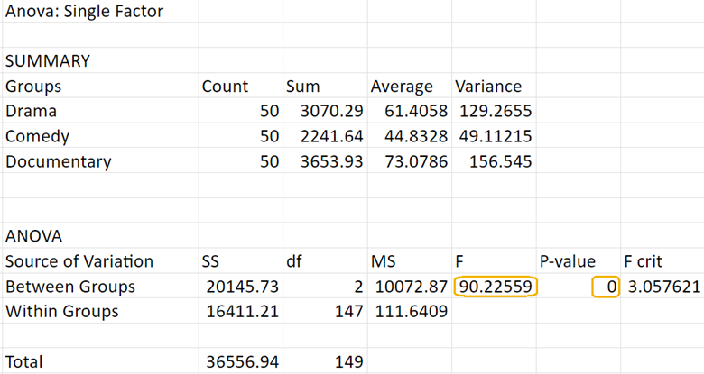
Since the p-value (<0.0001) is less than the significance level (0.05), you reject the null hypothesis. This means there is sufficient evidence to conclude that there are significant differences in the average watch times between the three genres (Drama, Comedy, and Documentaries).
-
Check out this video on performing an ANOVA test to address the business problem.
In this lesson, you learned how to test differences among three or more population means using an ANOVA analysis. An introduction to ANOVA was provided that explained the purpose and application, such as comparing the sales team’s performance. The tutorial outlined the steps in ANOVA, including stating hypotheses, gathering data, choosing a significance level, performing the statistical test, and interpreting results. An ANOVA example demonstrated the process using a real-world scenario where a social media company analyzed engagement for three types of posts: Memes, Educational, and Promotional. This example helped illustrate how ANOVA can be used in a real-world business scenario to make data-driven decisions about content strategy and engagement on social media platforms.